Week 2 in Plain Language: How a Transformer Decoder Writes, Keeps Its Place and Stays Stable
Explain-like-I'm-12 version of the full Week 2 notes. Exam wording lives in the exam-focused guide and the real routed questions in the Week 2 question bank. If attention is new to you, start with Week 1 in plain language. Everything sits under the Knowledge Map.
The big idea of Week 2. A Transformer that writes an answer (a translation, say) must obey one rule: when it writes word number \(t\), it may look at the source sentence and at its own earlier words, but never at the future words. Everything else this week is machinery that makes that rule workable: a mask to hide the future, a bridge to the source sentence, a tag for each word's position, shortcut wires and normalization so deep stacks train, and two training tricks.
Think of a student writing an essay answer while reading a question paper. The question paper is open (that is the source). The student's own page so far is visible. The lines they have not written yet do not exist. That is the whole decoder.
Notation used below: B = batch size, S = source length, T = target length, d = model width, f = feed-forward width, h = heads, V = vocabulary size.
1. Teacher forcing: practising with the answer key's previous words
While training, we know the correct target sentence. At each step the decoder is handed the correct previous words (the "gold prefix"), not whatever it guessed. The inputs are the target shifted right by one slot, with a start symbol in front, so a position never sees its own answer.
The executed example (08_teacher_forcing.py):
| What | Tokens |
|---|---|
| Gold target | [1, 2, 3, 4] |
| Teacher-forced decoder input | [0, 1, 2, 3] (0 = start symbol) |
| Free-running input (model feeds on its own guesses) | [0, 1, 7, 6] |
Why bother? Because with gold inputs, every position can be computed at the same time (that is why Section 2 needs a mask). At test time the gold sentence does not exist, so the model feeds on its own outputs, and one early mistake can leak into later inputs.
Mistakes people make.
- Believing teacher forcing removes the training-versus-inference mismatch. It does not; it only makes training fast and stable.
- Forgetting the shift. The input is
[BOS, y1, ..., y(T-1)], the labels are[y1, ..., yT].
Hand-check. Gold [A, B, EOS], the model wrongly predicts C at step 2. Under teacher forcing the input for step 3 is B, the gold token (exam guide question 1).
Where the exam asks this
- 2025 T3 Quiz 1, Q175: the model said "content" at step 2 but the gold word was "suis". Derived answer: C, "suis".
- 2025 T3 Quiz 1, Q177: derived answer A, feed the correct preceding target token.
- 2025 T3 End Term AN, Q25: derived answer B, the ground truth is unavailable during generation.
- Also routed here: 2024 T1 Quiz 1, Q192 (marked ambiguous in the bank, so no answer is quoted).
2. Masked (causal) self-attention: hiding the future
Self-attention scores every word against every other word. For the writer, scores toward later words are forbidden. We forbid them by writing \(-\infty\) into those score cells before the softmax. Then \(e^{-\infty}=0\), so those words get exactly zero weight and the remaining weights still add up to 1.
The mask for 4 words (1 = blocked), from 01_causal_mask.py:
[[0, 1, 1, 1],
 [0, 0, 1, 1],
 [0, 0, 0, 1],
 [0, 0, 0, 0]]
Row 1 sees only itself; row 4 sees everyone. Blocked cells: \(1+2+3=6=T(T-1)/2\) for \(T=4\). The diagonal is not blocked.
Hand-check. Scores [2, 1, 5, 3], only the first two keys visible. Masked row: [2, 1, -∞, -∞]. Weights \(=[e^2, e]/(e^2+e)\approx[0.7311, 0.2689, 0, 0]\).
The executed 4x4 run shows the same staircase shape, e.g. row 2 is [0.3100, 0.6900, 0, 0] and the summed future weight is exactly 0.0.
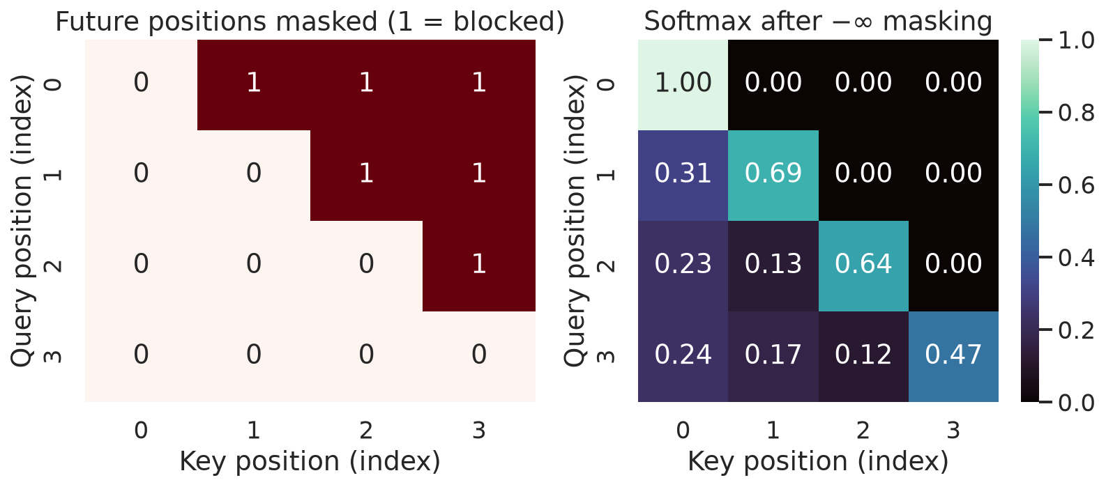
Figure 1. The blocked upper triangle receives zero probability after score masking; the visible probabilities are normalized within each row.
Mistakes people make.
- "The mask removes the diagonal." No: the diagonal is the current input, already a previous target. Only future positions are blocked.
- "Setting future values to zero is the same as masking." No: the future scores would still sit in the softmax denominator and shrink the visible weights. Mask the scores.
- A row with every key masked has no valid softmax; every valid query needs at least one visible key.
Where the exam asks this
- 2025 T3 Quiz 1, Q176: the row
[1, 2, 0, 2]for token 3. Derived answer C,[1, 2, 0, -∞]. - 2026 T2 Quiz 1, Q7: count the entries set to \(-\infty\) in a 128x128 mask. Derived answer 8,128, which is \(128\times127/2\).
- 2024 T3 Quiz 1, Q291: derived answer C, 64 x 64.
- 2026 T1 End Term AN, Q2: derived answer C, prevent target-future leakage.
3. Cross-attention: the decoder reading the source
In the decoder's second attention block the questions (queries) come from the decoder and the keys and values come from the encoder's final output. Each target word asks "which source words matter for me right now?"
Shapes (executed in 02_cross_attention_shapes.py, [B, S, T, d, h] = [2, 5, 3, 16, 4]):
| Piece | Shape |
|---|---|
| Decoder states (queries) | [2, 3, 16] |
| Encoder output (keys, values) | [2, 5, 16] |
| Attention weights, all heads | [2, 4, 3, 5] = [B, h, T, S] |
| Output | [2, 3, 16] |
Rule: rows come from the queries, columns from the keys. Three target words and five source words give a 3 x 5 table. No causal mask is applied over the source: the whole source sentence is already known. Only padding in the source is hidden.
Mistakes people make.
- Applying a causal mask to the source. Not needed in ordinary cross-attention.
- Thinking the decoder is "an encoder plus a mask". It has an extra sublayer, so it has an extra set of projections.
Where the exam asks this
- 2024 T1 Quiz 1, Q190 and 2025 T1 Quiz 1, Q104: attention-matrix size per head. Derived answer D, T2 x T1 in both.
- 2025 T3 Quiz 2, Q128: derived answer A, Q from the decoder, K and V from the encoder.
- 2026 T1 Quiz 1, Q5: derived answer C, no source causal mask; source padding may be masked.
4. The decoder's output layer and counting parameters
After the last decoder block, a final linear layer turns each position's vector ([B, T, d]) into one score per vocabulary word ([B, T, V]), then a softmax picks probabilities. The weight matrix is [d, V], so it has \(d\times V\) numbers, plus \(V\) if there is a bias.
Executed numbers: \(d=512\), \(V=37{,}000\) gives \(512\times37{,}000=18{,}944{,}000\) weights (plus \(37{,}000\) with a bias, 18,981,000 in total, from the exam guide).
Counting one decoder layer. With biases, one full-width attention block has \(4d^2+4d\) parameters, and a decoder layer has two of them (masked self-attention and cross-attention), one feed-forward net (\(2df+f+d\)) and three LayerNorms (\(6d\)):
| Size | Attention (x2) | Feed-forward | 3 LayerNorms | Total |
|---|---|---|---|---|
Tiny d=4, f=8 |
160 | 76 | 24 | 260 |
d=512, f=2048 |
2,101,248 | 2,099,712 | 3,072 | 4,204,032 |
The tiny row you can do by hand (attention: \(2\times(4\cdot16+16)=160\); FFN: \(2\cdot4\cdot8+8+4=76\); norms: \(6\cdot4=24\)). It was also checked against PyTorch's own TransformerDecoderLayer(4, 1, 8), which reports 260. The big row matches 07_decoder_parameter_count.py ("decoder layer formula=4,204,032; torch count=4,204,032; equal=True"). Six such layers give 25,224,192, leaving out embeddings and the output layer. The course shorthand "about 4M per layer" is a rounding of 4.204M.
Mistakes people make.
- Using a library total when the question says to exclude biases or embeddings. Follow the question's exclusions.
- Counting a shared (tied) weight twice.
- Counting an encoder layer with two attention blocks; it has one.
Where the exam asks this
- 2024 T3 Quiz 1, Q277, Q278, Q279 and Q280. Three of these are marked ambiguous in the bank because they depend on the bias and tying convention, so read the bank's notes rather than trusting one number.
5. Sinusoidal positional encoding: a tag for "where am I?"
Attention alone does not know word order: shuffle the input rows and the output rows just shuffle too. So we add to each word vector a position tag built from sines and cosines of different speeds:
Think of a clock with several hands: a fast second hand, a slower minute hand. Together they identify the time uniquely.
Hand-check, d=4. Here \(\omega_0=1\) and \(\omega_1=10000^{-1/2}=0.01\).
| Position \(p\) | \([\sin p,\ \cos p,\ \sin 0.01p,\ \cos 0.01p]\) |
|---|---|
| 0 | [0, 1, 0, 1] |
| 1 | [0.8415, 0.5403, 0.0100, 1.0000] |
Position 0 is always [0,1,0,1,...]. Every entry lies in \([-1,1]\), and the squared length of any tag is \(d/2\) (here 2). An independent implementation matched the formula to 0.00000011 (03_sinusoidal_pe.py).
The neat trick. Each sine-cosine pair at position \(p+k\) is a rotation of the pair at \(p\) by the angle \(k\omega_i\), and that rotation depends on the offset \(k\) only, not on \(p\). So "3 steps later" is the same simple linear map everywhere.
Mistakes people make.
- "Sinusoidal tags guarantee good length extrapolation." They can be computed for unseen positions, but whether the model uses them well is empirical.
- "Distance between tags grows steadily with the gap." It oscillates.
- Mixing up the coordinate index and the pair index \(i\), and forgetting that positions start at zero.
Where the exam asks this
- 2024 T1 Quiz 1, Q184: sum of the elements of \(P_5\) with dimension 2. Derived answer \(\sin 5+\cos 5\approx-0.675262\).
- 2025 T3 Quiz 1, Q174: derived answer C, sine in even dimensions and cosine in odd.
- 2026 T1 Quiz 1, Q12: a single cosine entry; the prompt's index is ambiguous, so see the bank.
- 2025 T2 Quiz 1, Q144, 2024 T3 Quiz 1, Q293: more arithmetic of the same kind.
6. Residual connections and normalization
Residual connection. Each sublayer's output is added to its own input: \(x+F(x)\). Like a shortcut staircase next to the winding path: the signal (and the gradient on the way back) always has a direct route. The two things added must have the same shape [B, T, d].
The original wiring (post-LN): \(z=\operatorname{LN}(x+\operatorname{Sublayer}(x))\), at each of the three decoder sublayers (masked self-attention, cross-attention, FFN).
LayerNorm rescales one token's d numbers to mean 0 and variance 1, then applies learned \(\gamma,\beta\):
Hand-check. \(x=(1,2,3)\): mean \(=2\), variance \(=(1+0+1)/3=2/3\), output \(=(-\sqrt{3/2},\,0,\,\sqrt{3/2})\approx(-1.2247,\,0,\,1.2247)\). The executed single-token run (04_norm_axes.py) printed exactly -1.2247, 0.0000, 1.2247.
BatchNorm instead normalizes each feature across the batch (and time). Take the batch \(X=\begin{bmatrix}1&2\\3&4\end{bmatrix}\) (rows = samples), \(\gamma=1,\beta=0,\epsilon=0\). Feature 1 has values 1 and 3: mean 2, standard deviation 1, giving \(-1\) and \(+1\). Same for feature 2. Result: \(\begin{bmatrix}-1&-1\\1&1\end{bmatrix}\). Doing LayerNorm on the same rows would instead normalize [1,2] and [3,4] separately, each to \((-1,+1)\).
| LayerNorm | BatchNorm | |
|---|---|---|
| Averages over | the d features of one token |
batch (and time), one feature at a time |
| Depends on other examples / padding? | No | Yes |
| Train vs evaluation | Same computation | Evaluation commonly uses running statistics |
| Why Transformers prefer it | Works for any batch size and sequence length | Statistics get contaminated by padding |
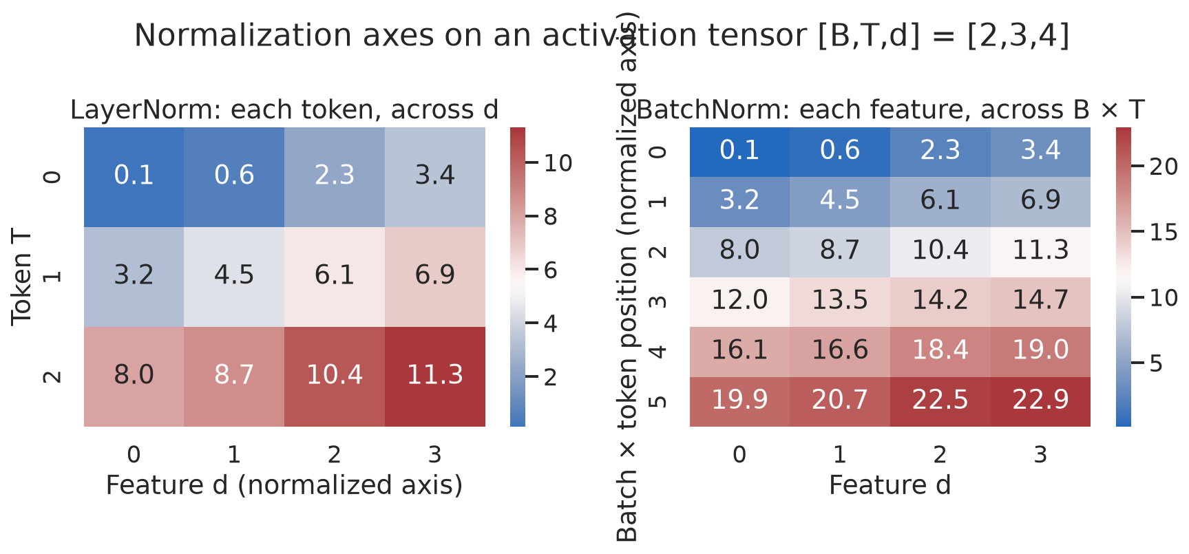
Figure 2. For [B,T,d]=[2,3,4], LayerNorm aggregates the four features of each token; BatchNorm pools batch and sequence observations for each feature.
Mistakes people make.
- "BatchNorm with one value returns the input." With a single observation the normalized value is zero (output is \(\beta\)), and PyTorch even raises an error: "Expected more than 1 value per channel when training".
- "Original BERT used pre-LN." It uses post-residual LayerNorm.
- "A residual connection guarantees gradients never vanish." It gives an extra path, not a guarantee.
Where the exam asks this
- 2025 T3 Quiz 1, Q179: the exact
[[1,2],[3,4]]example above. Derived answer A,[[-1,-1],[1,1]]. - 2026 T1 Quiz 2, Q12: LayerNorm of sample
[1,3,5,7]. Derived answer \(3/\sqrt5\approx1.341641\). - 2025 T3 Quiz 2, Q127: derived answer D, BatchNorm 1,024 and LayerNorm 1,024 parameters.
- 2024 T3 Quiz 1, Q281: a BatchNorm row sum (derived answer 0).
7. Training tricks: label smoothing and the warm-up schedule
Label smoothing. Instead of saying "the right word has probability 1 and all others 0", we say "right word about 0.9, the others share a little". It stops the model from becoming over-confident. With the uniform-mixture rule \(q_i=(1-\varepsilon)\mathbf 1[i=y]+\varepsilon/V\):
- Hand-check, \(V=5\), gold class 3rd, \(\varepsilon=0.1\): every class gets \(0.1/5=0.02\), the gold gets \(0.9\) extra, so
[0.02, 0.02, 0.92, 0.02, 0.02](sums to 1). - Executed (
05_label_smoothing.py, \(V=4\)): target[0.025, 0.025, 0.925, 0.025]; hand-built loss0.66827178equals PyTorch'slabel_smoothing=0.1loss (equal=True).
Another convention gives the gold exactly \(1-\varepsilon=0.9\); always say which one you use.
Warm-up schedule. Start the learning rate tiny, ramp it up linearly, then let it fall slowly:
Like warming up before a sprint. The peak is at \(s=w\). Executed values (06_warmup_schedule.py):
| Step | \(d=512\) | \(d=256\) |
|---|---|---|
| 1 | 0.0000001747 | 0.0000002471 |
| 1000 | 0.0001746928 | 0.0002470529 |
| 4000 (peak) | 0.0006987712 | 0.0009882118 |
| 8000 | 0.0004941059 | 0.0006987712 |
Hand-check: step 1000 is a quarter of the way up the ramp, so \(0.0006987712/4=0.0001746928\). Step 8000 is \(\sqrt{4000/8000}=1/\sqrt2\) of the peak.
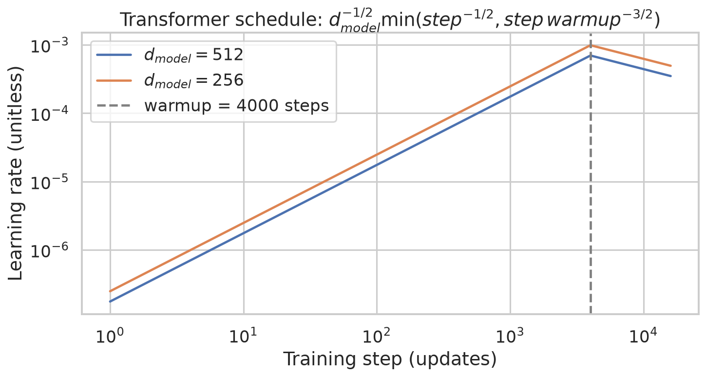
Figure 3. For widths 256 and 512, rates peak at step 4000 and decay thereafter; width 512 gives lower rates by a factor of \(1/\sqrt2\) at the same step.
Mistakes people make.
- Treating smoothed cross-entropy as ordinary negative log-likelihood.
- Thinking the schedule is the literal size of every weight update: Adam rescales each parameter.
- Claiming warm-up is a universal stability proof. It is a training choice.
Where the exam asks this
- 2025 T2 End Term FN, Q142: which are valid design choices of a transformer language model (learning-rate schedule and normalization type are among them). Derived answer A, B, D and E. This is the only routed question for this topic.
8. The full Transformer data flow
- Source tokens become embeddings plus position tags.
- Six encoder blocks (self-attention, then feed-forward), each wrapped in residual + LayerNorm, produce the "memory" of the source.
- Target tokens, shifted right, become embeddings plus position tags.
- Six decoder blocks, each with (a) masked self-attention, (b) cross-attention reading the encoder memory, (c) feed-forward, each wrapped in residual + LayerNorm.
- A linear layer to
[B, T, V], then softmax gives next-word probabilities.
Training runs all target positions in parallel (teacher forcing + mask). Generation appends one chosen word at a time until the end symbol or a length limit. Source and target may have different lengths.
Mistakes people make. Saying only the encoder gets position tags (both do), or that the decoder has no token embeddings (it does), or that the mask applies only in the first decoder layer (it applies in every decoder self-attention layer).
Where the exam asks this
- 2025 T3 Quiz 1, Q184: true statements about the architecture. Derived answer A, D and E.
- 2026 T2 Quiz 2, Q4, 2024 T3 End Term AN, Q191, 2024 T3 End Term FN, Q190.
The answers quoted above are derived study aids produced by the study team, not official answer keys. Where a record is marked ambiguous in the bank, no answer is quoted here.
Check yourself
- Gold target
[A, B, EOS]. What is the decoder's training input, and what does step 3 receive if step 2 was wrongly predicted asC? - In a 5-word causal mask, how many cells are set to \(-\infty\)?
- Three target words attend to six source words in one head. What is the shape of the weight table?
- What is \(PE(0)\) for \(d=4\)?
- Normalize
[1, 2, 3]with LayerNorm (\(\gamma=1,\beta=0\), ignore \(\epsilon\)). Then say what BatchNorm would do differently.
Answers
- Input
[BOS, A, B]; step 3 receivesB, the gold token. - \(5\cdot4/2=10\).
[3, 6]: rows from the decoder queries, columns from the encoder keys (per head, per batch item).[0, 1, 0, 1].- Mean 2, variance \(2/3\), output \((-1.2247,\,0,\,1.2247)\) computed within this single token. BatchNorm would instead normalize each feature across the whole batch (and time), so its answer depends on the other examples.
Bridge to Week 3
Week 2 completed the original encoder-decoder Transformer: hide the future, read the source, tag positions, keep layers stable, train smoothly. Week 3 in plain language builds on this decoder side of the design. For the formal treatment, return to Week 2: Transformer Decoding, Position, Normalization, and Training, Week 2: Transformer Decoder Exam-Focused Notes, Week 2: LLM Exam Questions and Worked Answers and the LLM Knowledge Map; the previous step is Week 1 in plain language: from one squeezed summary to attention and the Transformer encoder.