Week 4 in plain language: how a model picks words, and how BERT learns by filling blanks
Explain-like-I'm-12 version of the full Week 4 notes. Exam wording lives in the exam-focused guide and the Week 4 past-paper bank. Start from Week 3 in plain language if the idea of a model that predicts the next word is new. Hub: LLM Knowledge Map.
The big idea of Week 4. A language model never "writes" text. At each step it hands you a list of probabilities, one per word in its vocabulary. A decoding rule (greedy, beam, top-k, top-p, temperature) is the game plan for turning that list into actual words. Then we meet BERT, a model that learns the opposite way: instead of guessing the next word, it gets a sentence with some words hidden and learns to fill the blanks, using words on both sides.
1. Exhaustive and greedy search
The model gives \(P(y_t \mid x, y_{<t})\) at each step. The probability of a whole sentence is the product of the step probabilities (and the log of it is the sum of the logs).
- Exhaustive search tries every possible sentence. With a vocabulary of \(V\) tokens and length \(T\) there are \(V^T\) of them. With 6 tokens and length 5 that is \(6^5 = 7{,}776\). For \(40{,}000^5 = 1.024\times10^{23}\) sequences, at a billion per second the notes estimate about 3.24 million years. Far too slow for a real vocabulary.
- Greedy search always takes the single most likely next token and never looks back.
Hand-checkable trap (from the executed code, 01_decoding). First word: A has 0.51, B has 0.49. After A the best next word is b (0.6). After B the best next word is a (0.99).
| Path | Calculation | Probability |
|---|---|---|
| Greedy: A then b | \(0.51 \times 0.6\) | 0.3060 |
| Other: B then a | \(0.49 \times 0.99\) | 0.4851 |
Greedy grabbed the bigger first step and missed the better whole sentence. Counting tip: with 6 tokens, step 4 has \(6^3 = 216\) different three-token prefixes, and each needs one decoder run, so 216 evaluations (batching and EOS rules ignored).
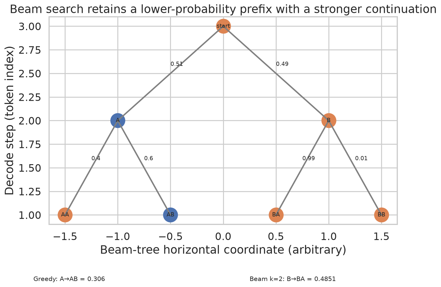
Figure 1. Greedy picks A then b (0.3060); a width-two beam keeps B alive and finds B then a (0.4851).
Mistakes people make. "Greedy gives the most probable sentence" is false, because the next distribution depends on the prefix you chose. Also, a candidate expansion and a model call are different counts: for \(V=3\), \(T=2\) there are nine two-token candidates but only \(1+3\) prefix evaluations.
Where the exam asks this: 2025 T2 Quiz 1, Q153 (decoder runs at step 4), 2025 T2 Quiz 1, Q154 (length-5 sequences), 2025 T3 Quiz 1, Q178 (sequences up to length 5), 2025 T3 Quiz 1, Q180 (extra sequences when \(L\) becomes \(L+1\)), 2024 T1 End Term AN, Q148 (greedy on a probability table). Derived study answers: 216, 7,776, \(\sum_{k=1}^{5}|V|^k\), and \((V-1)V^L\).
2. Beam search and length normalisation
Beam search is greedy with a safety net. Keep the best \(b\) unfinished sentences (the "beam width"), extend each by every word, score all the results, and keep the best \(b\) again.
Worked example, same tree as above, \(b=2\):
- Step 1: keep both A (0.51) and B (0.49).
- Step 2: candidates are Aa \(=0.51\times0.4\), Ab \(=0.306\), Ba \(=0.4851\), Bb \(=0.49\times0.01\). The best two are Ba and Ab.
The code works in log scores (adding is easier than multiplying): \(\log 0.4851 = -0.7234\) and \(\log 0.3060 = -1.1842\). With \(b=1\) beam equals greedy (same rules for ties and stopping). A bigger beam is not automatically exhaustive, because it still prunes at later depths.
Length problem. Each extra word multiplies by a number below 1, so long sentences look worse just for being long. Length normalisation divides the log score by \(\ell^\alpha\) (\(\ell\) = length). Tiny example from the notes: one-token score \(-1.0\), three-token score \(-1.5\).
| Candidate | Raw score | Mean score (\(\alpha=1\)) |
|---|---|---|
| 1 token | \(-1.0\) | \(-1.0\) |
| 3 tokens | \(-1.5\) | \(-1.5/3 = -0.5\) |
Raw ranking prefers the short one; mean ranking prefers the long one. Normalising changes the goal; it is a heuristic. In the equal-length tree above (both candidates have length 2), dividing by 2 changes nothing about who wins.
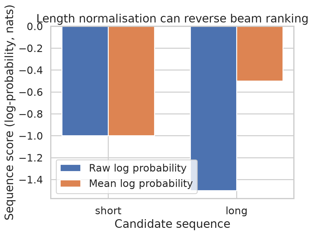
Figure 2. Raw scores favour the one-token candidate (\(-1.0\) over \(-1.5\)); mean scores flip the order (\(-0.5\) over \(-1.0\)).
Where the exam asks this: 2025 T3 Quiz 1, Q181 (how many beams at step 1 and step 3 for greedy, beam size 3, exhaustive; derived answer D: 1, 3, 10 after one step and 1, 3, 1000 after three), 2026 T2 Quiz 1, Q17 (smallest beam width that keeps a given path; derived answer 5, because the path's rank must be within the width at every step), 2026 T2 End Term AN, Q4.
3. Top-k sampling and temperature
Sampling means rolling a weighted die instead of taking the maximum.
Top-k: keep only the \(k\) most likely tokens, set the rest to zero, then renormalise (divide by what is left so they sum to 1).
Example from the code, \(p=(0.42, 0.25, 0.15, 0.10, 0.08)\) for tokens A to E, \(k=3\): kept mass \(0.42+0.25+0.15=0.82\), so the new probabilities are \(0.42/0.82, 0.25/0.82, 0.15/0.82 = (0.5122, 0.3049, 0.1829)\). The program prints exactly [0.5122 0.3049 0.1829 0. 0.].
Temperature \(\tau\) divides the logits before softmax: \(p_i = e^{z_i/\tau}/\sum_j e^{z_j/\tau}\). Low \(\tau\) makes the favourite stronger (sharper); high \(\tau\) evens things out (flatter). Positive temperature never changes the ranking. Example with logits \((2,1,0,-1)\):
| \(\tau\) | \(p\) for the four tokens | Entropy (nats) |
|---|---|---|
| 0.5 | 0.8650, 0.1171, 0.0158, 0.0021 | 0.455 |
| 1 | 0.6439, 0.2369, 0.0871, 0.0321 | 0.948 |
| 2 | 0.4551, 0.2760, 0.1674, 0.1015 | 1.245 |
(Entropy = "how unsure the distribution is"; it rises with temperature, matching Figure 3. The probability columns are tiny calculations checked with uv run python.) The script's five-token example (different numbers!) prints entropy 1.0341, 1.4278, 1.5623 for \(\tau = 0.5, 1, 2\).
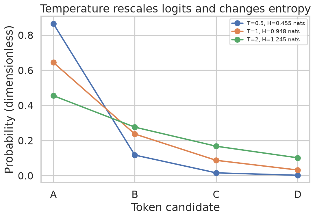
Figure 3. For logits \((2,1,0,-1)\), entropy rises from 0.455 nats at \(\tau=0.5\) to 0.948 at \(\tau=1\) and 1.245 at \(\tau=2\).
Mistakes people make. "\(\tau=2\) is low temperature" is false: relative to \(\tau=1\) it flattens. "Sampling gives a different answer every time" is false: identical draws are possible, and a fixed seed repeats a run. Seeing repeated output does not tell you which algorithm made it.
Where the exam asks this: 2026 T1 Quiz 2, Q17 (top-2 renormalise: \(0.4/0.65 \approx 0.62\), derived), 2025 T2 Quiz 1, Q145 (temperature 0.5 on logits \(2, 1, 0.5, -1\); derived about 0.84), 2025 T2 Quiz 1, Q155 (top-2 renormalised, derived about 0.411), 2025 T3 End Term AN, Q2 (temperature plus top-2: apple or banana, because dividing by a positive number keeps the order).
4. Top-p (nucleus) sampling and repetition problems
Top-p keeps the smallest group of top tokens whose total probability reaches at least \(p\) (including the token that crosses the line), then renormalises. The group size adapts: when the model is sure, the nucleus is small; when it is unsure, it is large.
Using the same \(p\) vector with \(p_{\text{threshold}} = 0.80\): cumulative sums \(0.42, 0.67, 0.82\), so keep three tokens. That is why top-p and top-3 give the same result in the code. Another hand check from the notes: \((0.5, 0.2, 0.15, 0.1, 0.05)\) at 0.8 has cumulative sums \(0.5, 0.7, 0.85\), keep 3, and the first token becomes \(0.5/0.85 = 10/17 \approx 0.5882\).
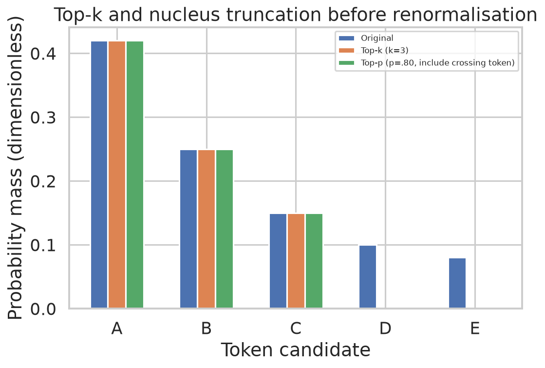
Figure 4. Top-3 and top-\(p=0.80\) both keep original mass \(0.42+0.25+0.15=0.82\) before renormalising.
Repetition. Always chasing the highest probability tends to give repetitive, generic text, while sampling from the whole vocabulary can wander into a junk tail. Holtzman et al. (2020) proposed nucleus sampling to cut the tail adaptively. It does not guarantee truth or no repetition. Flattening with a high temperature first can enlarge the nucleus.
Mistakes people make. "\(p=1\) is a mistake" is wrong: it keeps everything with positive probability. And "exceeds the threshold" does not mean you must drop a token that lands exactly on \(p\): the convention here is "at least \(p\)". Always check the convention a question states.
Where the exam asks this: 2025 T2 End Term AN, Q198 (nucleus size for ten probabilities at \(p=0.7\): sorted sums 0.20, 0.35, 0.49, 0.60, 0.69, 0.77, so 6 tokens, derived), 2026 T1 End Term AN, Q8 (3 tokens, derived), 2025 T3 Quiz 1, Q182 (which strategy is inherently random: nucleus, derived), 2026 T2 Quiz 2, Q10 (temperature 5 before top-p; derived answer A, the nucleus tends to grow, though it can stay equal).
5. BERT and masked language modelling
GPT reads left to right and predicts the next word, so it can only see the past (a causal mask). BERT sees the whole sentence at once and learns by hiding words. That makes it bidirectional: to guess a blank it uses words on both sides.
The recipe. Pick 15% of word positions. For the picked positions only:
| What happens to a picked position | Share of picked | Share of all positions |
|---|---|---|
Replace with [MASK] |
80% | 12% |
| Replace with a random word | 10% | 1.5% |
| Leave unchanged | 10% | 1.5% |
Check by hand with 1,000 positions: \(1000 \times 0.15 = 150\) picked, so 120 masks, 15 random, 15 unchanged. The model is graded on all 150 picked positions, including the unchanged ones. Why leave some alone or random? So the model cannot learn "only look hard when I see [MASK]", since [MASK] never appears when BERT is used later.
The executed simulation (1,000,000 positions, seed 42) found 14.9892% picked, then 79.9322% mask, 10.1320% random, 9.9358% unchanged among the picked: close to the recipe but not exact, because it is random.
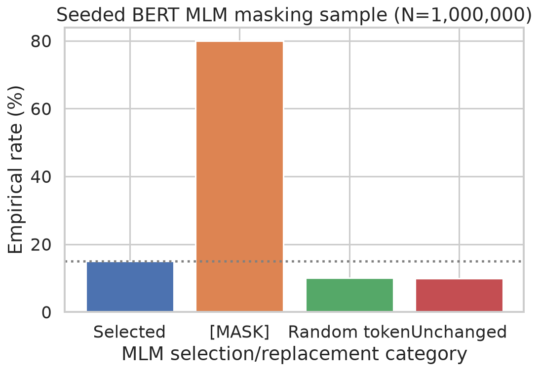
Figure 5. The seeded million-position simulation selects 14.989% of positions; of those, about 79.93% mask, 10.13% random and 9.94% unchanged.
Mistakes people make. "80/10/10 is a share of all tokens" is false; it is a share of the picked 15%. "Hiding the position in attention is enough" is false: residual connections carry the original token forward, so BERT corrupts the input instead. [MASK] is also not the padding mask, which is a separate attention mask.
Where the exam asks this: 2026 T1 Quiz 2, Q3 (why keep 10% unchanged; derived answer C: it reduces the mismatch between pre-training and later use), 2026 T1 Quiz 2, Q4 (why plain GPT does not suit BERT-style MLM: the causal mask blocks right-hand context; derived answer B).
6. Next sentence prediction, [CLS], [SEP] and the three embeddings
NSP is a second game: given sentences A and B, is B the real next sentence? Half the training pairs are real neighbours, half use a random sentence for B. The code builds exactly 50.0% consecutive and 50.0% random-next. The label describes how the pair was built; a random B could coincidentally fit.
The input looks like this (from the executed code):
| Token | [CLS] |
A1 | A2 | [SEP] |
B1 | B2 | [SEP] |
|---|---|---|---|---|---|---|---|
| Segment id | 0 | 0 | 0 | 0 | 1 | 1 | 1 |
[CLS]is a summary slot; its final vector feeds the yes/no classifier (and later, classification tasks).[SEP]marks a boundary.- Every position gets three embedding vectors, each of shape
[H], that are added (not joined): token + position + segment. The batch input is[B, T, H].
Mistake box. Summing is not concatenating. Segment ids say "part A or part B", they do not make attention one-directional. NSP is classification, not generation.
Where the exam asks this: 2025 T2 Quiz 1, Q142 (which items are in the NSP input: [CLS], [SEP], segment embeddings; derived A, B, C, and position embeddings are also part of the input), 2026 T1 End Term FN, Q6 (how negative pairs are made: pick another sentence from the corpus at random; derived C).
7. BERT sizes and parameter counts
| Layers \(L\) | Hidden \(H\) | Heads | FFN width \(I\) | Paper headline | |
|---|---|---|---|---|---|
| BERT-base | 12 | 768 | 12 | 3072 | about 110M |
| BERT-large | 24 | 1024 | 16 | 4096 | about 340M |
The executed count (formula and real PyTorch modules agree) covers the three embedding tables, the embedding LayerNorm, all encoder layers and the pooler. It does not include the extra pre-training heads. With a vocabulary of 30,522:
- BERT-base: 109,482,240
- BERT-large: 335,141,888
Vocabulary caveat. The paper describes a 30,000-token vocabulary; the standard released model has 30,522. With 30,000 the same count gives 109,081,344 (base) and 334,607,360 (large). The 522 extra rows add \(522 \times 768 = 400{,}896\) and \(522 \times 1024 = 534{,}528\) parameters, and \(109{,}081{,}344 + 400{,}896 = 109{,}482{,}240\) checks out. The headline "110M / 340M" is a rounded figure, not an exact count.
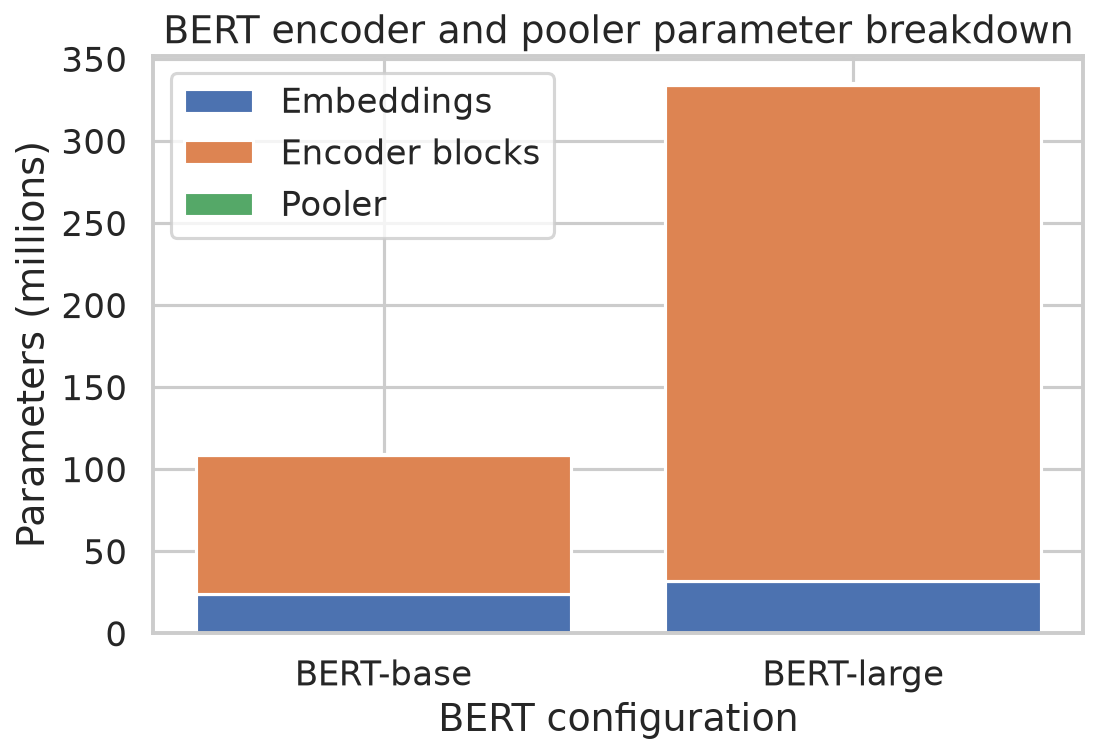
Figure 6. Embeddings, encoder and pooler total 109,482,240 (base) and 335,141,888 (large); the paper rounds these to about 110M and 340M.
Hand-checkable mini version (exam style, embedding tables only): \(V=5000\), \(P=64\), \(S=2\), \(H=128\) gives \((5000+64+2)\times128 = 648{,}448\). Add \(2\times128 = 256\) for the embedding LayerNorm if asked, giving 648,704.
Where the exam asks this: 2026 T1 Quiz 2, Q18 (embedding layer of a small BERT-like model; derived 648,448, the numbers above), 2024 T1 End Term FN, Q198 (what BERT stands for; derived B).
8. Fine-tuning heads and GPT versus BERT
After pre-training, you bolt a small head on top and train it for a task. Let the final encoder output be [B, T, H].
| Task | What the head reads | Output shape or rule |
|---|---|---|
| Sentence classification (one label) | the final [CLS] vector |
[B, C] logits, softmax |
| Several labels at once (multilabel) | the final [CLS] vector |
one sigmoid per label |
| Entity tagging (NER) | every token vector | [B, T, C], ignore padding in the loss |
| Extractive question answering | every passage token | start score and end score per position, pick a span with start \(\le\) end |
Frozen features train only the head; full fine-tuning also updates BERT. Neither is guaranteed to win.
| GPT-style decoder | Original BERT | |
|---|---|---|
| Attention | causal, past only | both directions |
| Pre-training | next-token prediction | MLM plus NSP |
| Typical use | generate text | vectors for classification, tagging, spans |
Link-counting check: with length 5 per layer, free attention has \(5^2=25\) pairs and causal attention has \(5\cdot6/2=15\). Over 6 layers that is 150 versus 90. Same-size headline numbers (GPT-1 about 117M, BERT-base about 110M) do not mean the same objective.
Where the exam asks this: 2025 T3 End Term AN, Q5 (four-class task: use [CLS] plus a classifier; derived B), 2025 T3 End Term AN, Q6 (extract disease names: NER; derived C), 2025 T3 End Term FN, Q6 (multiple topics per abstract: a sigmoid per label; derived B), 2026 T1 End Term FN, Q17 (BERT 150 versus GPT 90; derived A).
The answers quoted above are derived study aids, not official answer keys. Where a question's record is marked ambiguous, this note does not state an answer.
Check yourself
- Greedy picks A (0.51) then b (0.6); another path is B (0.49) then a (0.99). Which whole sentence is more probable?
- Top-2 on \((0.40, 0.25, 0.20, 0.10, 0.05)\): what is the new probability of the first token?
- In 1,000 eligible positions, how many are expected to be (a) picked, (b) turned into
[MASK], (c) left unchanged but still graded? - For logits \((2,1,0,-1)\), does \(\tau=2\) make the top token more or less likely than \(\tau=1\)? Give both numbers.
- Why do the BERT-base totals 109,482,240 and 109,081,344 differ, and which does the paper's 30,000 vocabulary match?
Answers
- B then a: \(0.49\times0.99=0.4851\) beats \(0.51\times0.6=0.3060\).
- Kept mass \(0.65\), so \(0.40/0.65 = 8/13 \approx 0.6154\).
- (a) 150; (b) 120; (c) 15. These are expectations, not guaranteed counts.
- Less likely: 0.6439 at \(\tau=1\) falls to 0.4551 at \(\tau=2\), because \(\tau=2\) flattens the distribution.
- The larger number uses 30,522 vocabulary rows; the 522 extra rows add \(522\times768=400{,}896\) parameters. The paper's 30,000-token vocabulary corresponds to 109,081,344.
What comes next
Everything so far assumed a model that is already trained, and it only decided how to read out words or how to pre-train. Later parts of the course move on to other topics, which are not assumed here. For now, remember the two pictures: a probability list plus a decoding rule gives text, and hidden-word guessing gives BERT its two-sided understanding.
Back to Week 3 in plain language · Full notes · Exam-focused guide · Past-paper bank · LLM Knowledge Map