Week 1: From Sequence Models to Transformer Encoders
Read the Week 1 plain-language (ELI12) note first, then come back here.
Learn and revise for the exam: Week 1 exam guide · Routed questions and worked answers
Navigation: Knowledge Map · Week 2 Notes →
Abstract
Fixed-context recurrent encoder–decoders compress a source sequence into one representation, creating an information bottleneck and sequential computation. Additive attention replaces that single source summary with a decoder-step-dependent weighted combination of encoder states. Transformer self-attention constructs contextual representations by learned query, key and value projections, scaled dot products, and normalized value aggregation. Multiple heads apply distinct projections before concatenation and an output projection; a position-wise feed-forward network and post-normalized residual connections complete the original encoder layer. A parameter audit distinguishes weights, optional biases and normalization from sequence-length-dependent activations.
Lecture map and question routing
The ebook transcript covers PDF pp. 4–20 (printed pp. 3–19). Page references below identify both numbering systems. The following table lists every record routed to Week 1; records with multiple topic IDs appear in each applicable row. Question bank anchors identify source records, rather than substituting generated examples for examination questions.
1. From fixed context to attention
A sequence transducer estimates \(p(y\mid x)=\prod_t p(y_t\mid y_{<t},x)\). An early recurrent encoder–decoder replaces source access with a fixed-width \(c\), yielding \(p(y\mid x)=\prod_t p(y_t\mid y_{<t},c)\). The final state must transmit information relevant to all target positions. Long or information-rich inputs can therefore stress this channel; degradation is not inevitable at a particular length. Recurrent states also depend on their predecessors, limiting parallelism along time and making long gradient paths difficult (ebook PDF pp. 4–5 / printed pp. 3–4; Sequence-to-Sequence Bottleneck).
The Dangerous Misconception: Seq2seq means exactly two RNNs and a fixed vector. Why this is false: Seq2seq describes an input-to-output sequence mapping; attention-based recurrent models and Transformer encoder–decoders are also sequence-to-sequence models. The ebook's definition is narrower than the architecture family.
Bahdanau alignment
Given bidirectional encoder annotations \(h_i\) and previous decoder state \(s_{t-1}\), the learned additive score, normalized alignment and context are
The alignment matrix is [T_target, T_source]; every row sums to one over source positions. Its entries can be computed in parallel for a fixed decoder step, but the recurrent state makes successive decoder steps dependent. Different rows may favor different source positions; a diagonal pattern is not required when word order changes. A weight is a learned soft alignment, not a guaranteed causal explanation (PDF pp. 5–6 / printed pp. 4–5; Bahdanau Attention).
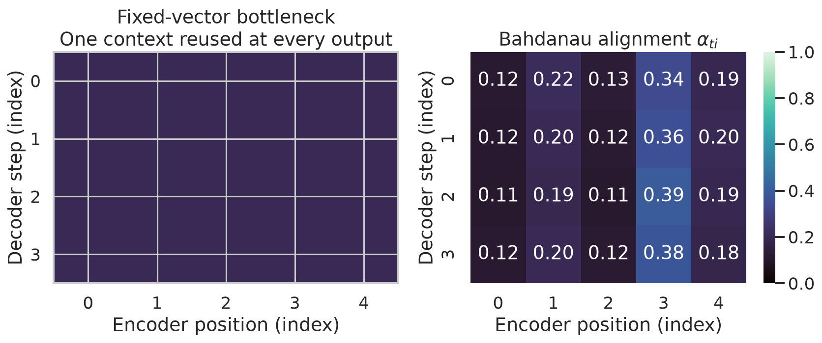
Figure 1. The left panel reuses a uniform context distribution at each output step; the right panel computes a separate additive alignment per decoder step using randomly sampled weights. These are illustrative distributions, not trained alignments or translation accuracy measurements.
2. Self-attention and scaled dot products
For row-oriented input \(X\) of shape [B, T, d_model], shared projections within a head give \(Q=XW^Q\), \(K=XW^K\), \(V=XW^V\). Their shapes are [B, T, d_k], [B, T, d_k], [B, T, d_v], with projection shapes [d_model, d_k], [d_model, d_k], [d_model, d_v]. The query requests information, a key determines compatibility, and a value supplies the content aggregated. Self-attention uses the same sequence for all three inputs; cross-attention uses a different source for keys and values. Learned matrices are distinct in the standard architecture (PDF pp. 6–8 / printed pp. 5–7; Self-Attention).
In the general case Q [B, T_q, d_k], K [B, T_k, d_k], V [B, T_k, d_v], \(A\) is [B, T_q, T_k] and \(Z\) is [B, T_q, d_v]. A mask \(M\) adds \(-\infty\) to forbidden logits before softmax; each query must retain an eligible key. Encoder self-attention normally permits all non-padding positions, including the query position itself. Without positional information or an order-dependent mask, self-attention is permutation equivariant, so content alone cannot encode order.
For a worked example, let \(d_k=1\), \(q=1\), \(k_1=k_2=0\), \(v_1=[1,0]\), \(v_2=[0,2]\). The two scaled scores are \([0,0]\), softmax gives \([1/2,1/2]\), and \(z=\frac12[1,0]+\frac12[0,2]=[0.5,1]\). The sum is over values, not keys.
Mathematical formulation: If the coordinates \(q_i,k_i\) are independent zero-mean, unit-variance variables, then \(\operatorname{Var}(q_i k_i)=1\) and independent products give \(\operatorname{Var}(q\cdot k)=d_k\). Dividing by \(\sqrt{d_k}\) gives variance one under these assumptions. This reduces growth of logit spread and mitigates softmax saturation; trained projections need not satisfy the assumptions, so scaling does not guarantee unsaturated gradients (PDF pp. 8–9 / printed pp. 7–8; Scaled Dot-Product Attention).
The Dangerous Misconception: Scaling makes every attention row uniform. Why this is false: Scaling changes the logit magnitudes, not their order; unequal logits generally give unequal weights. It is not a normalization across keys; softmax performs that step.
The Dangerous Misconception: The ebook's two displayed row and column input conventions produce transposed outputs. Why this is false: Transposing the input matrices in its PDF p. 8 / printed p. 7 expressions gives the same row-oriented output \(AV\); transposing the output would produce a column-oriented output. The paper's row convention is used throughout these notes.
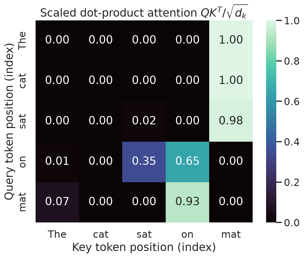
Figure 2. Each query row sums to one after softmax; cells show the normalized weight assigned to each key token in the five-token toy example.
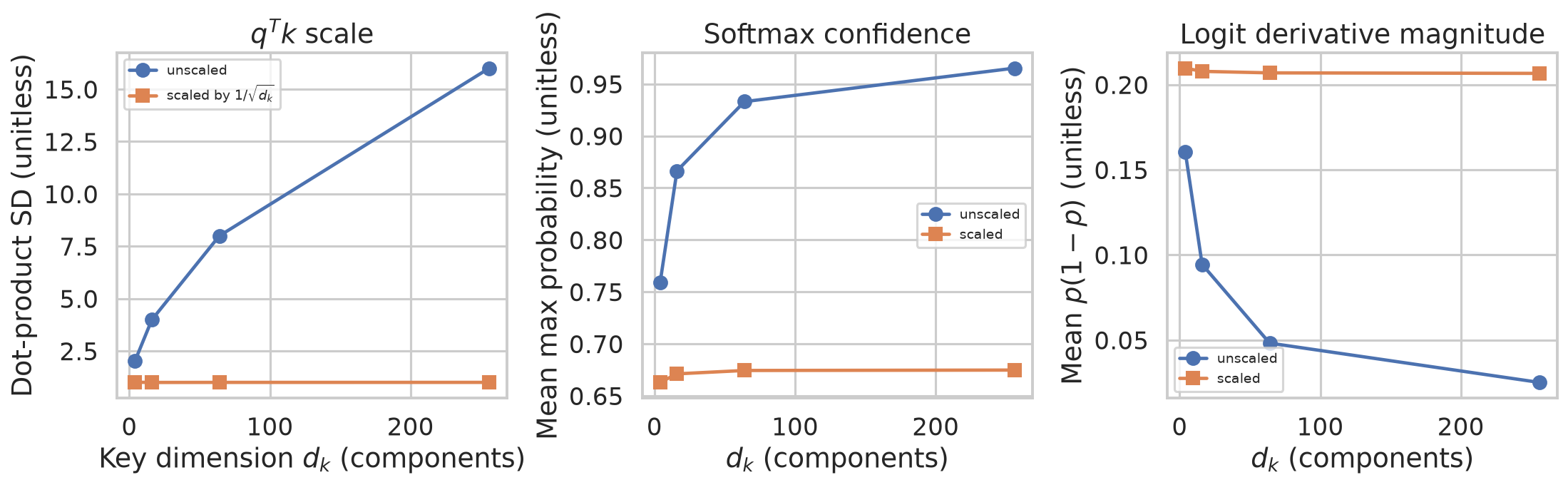
Figure 3. In the plotted random-vector experiment, unscaled dot-product spread grows with \(d_k\), whereas division by \(\sqrt{d_k}\) keeps its standard deviation near one and delays softmax saturation.
3. Multi-head attention and encoder architecture
Each head has independent projections. For self-attention,
For the original base model \(d_{\rm model}=512\), \(h=8\), \(d_k=d_v=64\). Each head is [B, T, 64], their concatenation is [B, T, 512], and \(W^O\) is [512, 512]. More generally the concatenation width is \(h d_v\) and \(W^O\) maps [h*d_v, d_model], mixing head features and restoring the residual width. The heads can learn different relations, but distinct or interpretable specializations are not guaranteed (PDF pp. 9–10 / printed pp. 8–9; Multi-Head Attention).
The Dangerous Misconception: With row-oriented head outputs the paper applies \(W^O\) on the left. Why this is false: It multiplies the concatenated row vectors on the right. The ebook's PDF p. 9 / printed p. 8 expression mixes conventions; its left multiplication requires a consistently transposed column-oriented representation.
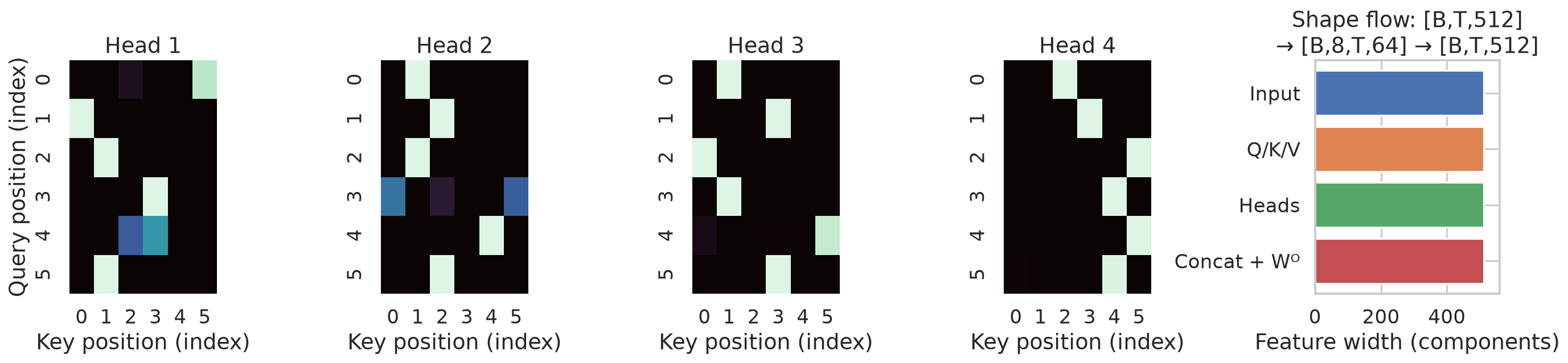
Figure 4. Four random attention patterns illustrate distinct heads; in the separate base-width schematic, eight 64-wide heads concatenate to 512 features. The four displayed patterns are illustrative, not a claim that four 64-wide heads yield 512 features.
Position-wise FFN and post-norm residuals
For each row \(x\), the original position-wise network is
where \(W_1\) is [d_model, d_ff] and \(W_2\) is [d_ff, d_model]. The same weights apply independently at every position in a layer, but different layers have separate parameters. Attention exchanges information between positions; the FFN mixes features at each position. Its ReLU makes the two affine maps more expressive than one affine map (PDF p. 10 / printed p. 9; Position-Wise Feed-Forward Network).
The original paper uses post-LayerNorm (dropout omitted here for clarity):
The residual additions require matching widths. LayerNorm operates over the feature dimension at each position. Six separately parameterized base encoder layers preserve [B, T, 512]; positions are processed in parallel within a layer, but successive layers depend on the previous output. Original encoder input includes embeddings plus positional encodings; decoder cross-attention and positional details are developed in Week 2: Transformer Decoding, Position, Normalization, and Training.
The Dangerous Misconception: The FFN directly attends to neighboring tokens. Why this is false: It is applied independently at each position; cross-token interaction comes from attention. The ebook's displayed \(W_1x\) is incompatible with its stated row-oriented [d_model, d_ff] matrix: the correct expression is \(xW_1\).
4. Encoder parameter accounting and computational cost
Set \(d=d_{\rm model}\) and \(f=d_{\rm ff}\), with \(hd_k=hd_v=d\). Q, K and V weights each total \(d^2\) over heads; output projection adds \(d^2\). The FFN contributes \(df+fd\) weights and \(f+d\) biases. Therefore
If all four attention projections have biases, add \(4d\); two affine LayerNorms add \(4d\). Thus the executable PyTorch convention is \(4d^2+2df+f+9d\). With \(d=512,f=2048\), its MHA has \(1{,}050{,}624\) parameters, FFN \(2{,}099{,}712\), two norms \(2{,}048\), and layer total \(3{,}152{,}384\). This excludes embeddings, position representations and task heads. A six-layer stack of independently parameterized layers contains \(6\times3{,}152{,}384=18{,}914{,}304\) under these assumptions. Fixed sinusoidal positions add no learned table; learned positional embeddings do. The ebook's “1M + 2M ≈ 3M” is a mnemonic, not an exact count (PDF pp. 10–11, 19–20 / printed pp. 9–10, 18–19; Encoder Layer Parameter Count).
The Dangerous Misconception: Increasing \(h\) at fixed \(d\) necessarily adds projection weights. Why this is false: With standard head widths \(d/h\), \(h(d\cdot d/h)=d^2\) per projection. \(W^O\) is not inherently an extra cost relative to a single-head layer: a single head may also have one. Count precisely what a question includes. The ebook's PDF p. 12 / printed p. 11 comparison omits this qualification.
Dense self-attention stores [B, h, T, T] scores, and score formation and value aggregation each require quadratic work in \(T\) at fixed width. FFN computation grows linearly in \(T\) at fixed dimensions. Doubling \(T\) quadruples score entries but does not alter shared layer weights. The projections themselves also cost computation; attention is parallel across positions but not free of quadratic memory or work.
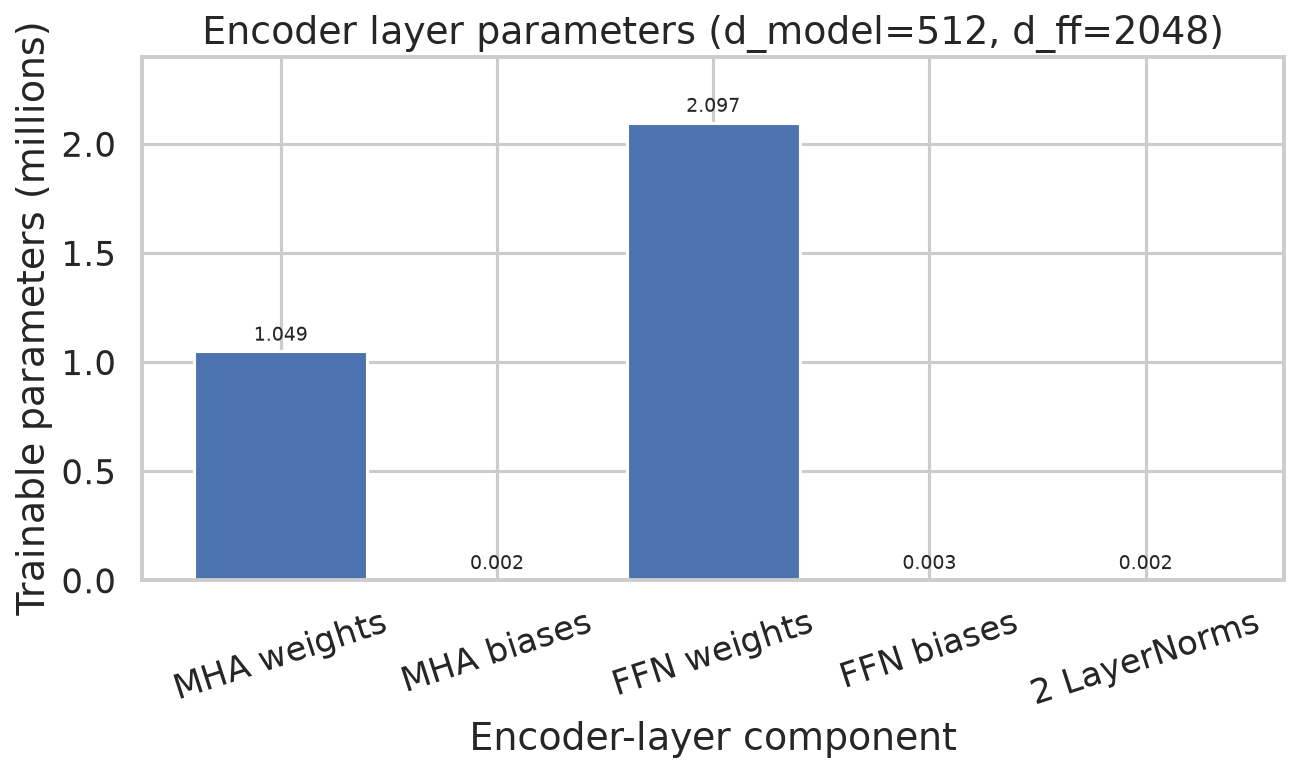
Figure 5. For \(d_{\rm model}=512\) and \(d_{\rm ff}=2048\), the plotted FFN parameter group exceeds the MHA group, while the two normalization groups are comparatively small.
5. Concept → Code → Output → Interpretation
The following complete scripts and outputs are reproduced verbatim from the executed Week 1 materials. Run each from LLM/ with uv run python 'week 1/codeblocks/<file>.py'; the recorded outputs describe the supplied environment and floating-point results can vary across environments.
5.1 01 Attention From Scratch
Concept
Scaled attention computes normalized rows and a value mixture.
Code
import numpy as np
import torch
import torch.nn.functional as F

rng = np.random.default_rng(42)
torch.manual_seed(42)
q = rng.normal(size=(1, 2, 3, 4)).astype(np.float32)
k = rng.normal(size=(1, 2, 5, 4)).astype(np.float32)
v = rng.normal(size=(1, 2, 5, 4)).astype(np.float32)
scores = q @ np.swapaxes(k, -1, -2) / np.sqrt(q.shape[-1])
z = scores - scores.max(axis=-1, keepdims=True)
a = np.exp(z) / np.exp(z).sum(axis=-1, keepdims=True)
y = a @ v
yt = F.scaled_dot_product_attention(torch.tensor(q), torch.tensor(k), torch.tensor(v))
print(f"attention shape={y.shape}; row-sum range={a.sum(-1).min():.6f}..{a.sum(-1).max():.6f}")
print(f"max |NumPy - torch SDPA|={np.max(np.abs(y-yt.numpy())):.8f}")
Output
attention shape=(1, 2, 3, 4); row-sum range=1.000000..1.000000
max |NumPy - torch SDPA|=0.00000011
Interpretation
The row sums are one to the shown precision and the NumPy result agrees with PyTorch SDPA to the reported floating-point tolerance.
5.2 02 Dot Product Variance
Concept
Independent random coordinates test the variance argument.
Code
import numpy as np
rng = np.random.default_rng(42)
for d in (4, 16, 64, 256):
    q = rng.normal(size=(20000, d))
    k = rng.normal(size=(20000, d))
    dot = np.sum(q*k, axis=1)
    print(f"d_k={d:3d} Var(q.k)={np.var(dot):8.2f} target={d:3d} scaled_var={np.var(dot/np.sqrt(d)):.3f}")
Output
d_k=  4 Var(q.k)=    4.04 target=  4 scaled_var=1.011
d_k= 16 Var(q.k)=   15.87 target= 16 scaled_var=0.992
d_k= 64 Var(q.k)=   63.83 target= 64 scaled_var=0.997
d_k=256 Var(q.k)=  253.99 target=256 scaled_var=0.992
Interpretation
The unscaled empirical variance increases with width; the scaled estimates remain close to one for this seeded sample.
5.3 03 Multihead Shape Check
Concept
Head splitting and output projection are checked against a standard module.
Code
import torch
import torch.nn as nn

torch.manual_seed(42)
B, T, D, H = 2, 5, 16, 4
x = torch.randn(B, T, D)
layer = nn.MultiheadAttention(D, H, dropout=0.0, batch_first=True)
q, k, v = [x @ layer.in_proj_weight[i*D:(i+1)*D].T + layer.in_proj_bias[i*D:(i+1)*D] for i in range(3)]
dh = D // H
split = lambda a: a.reshape(B, T, H, dh).transpose(1, 2)
qh, kh, vh = map(split, (q, k, v))
weights = torch.softmax(qh @ kh.transpose(-2, -1) / dh**0.5, dim=-1)
heads = (weights @ vh).transpose(1, 2).reshape(B, T, D)
y_manual = heads @ layer.out_proj.weight.T + layer.out_proj.bias
y_torch, _ = layer(x, x, x, need_weights=False)
print(f"input [B,T,d_model]=[{B},{T},{D}]")
print(f"heads [B,h,T,d_k]=[{B},{H},{T},{dh}]; concat={list(heads.shape)}")
print(f"max |manual - torch.nn.MultiheadAttention|={(y_manual-y_torch).abs().max().item():.8f}")
Output
input [B,T,d_model]=[2,5,16]
heads [B,h,T,d_k]=[2,4,5,4]; concat=[2, 5, 16]
max |manual - torch.nn.MultiheadAttention|=0.00000009
Interpretation
Four heads of width four concatenate to width sixteen; the reported discrepancy is a floating-point comparison, not an exact symbolic identity.
5.4 04 Encoder Parameter Count
Concept
An explicit formula includes attention biases and affine normalization.
Code
import torch.nn as nn

d, h, ff = 512, 8, 2048
# Formula matches PyTorch's combined QKV projection, biases, output projection,
# two FFN biases, and two affine LayerNorms (eps=1e-5, post-norm).
mha = 4*d*d + 4*d
ffn = 2*d*ff + ff + d
norms = 4*d
formula = mha + ffn + norms
layer = nn.TransformerEncoderLayer(d_model=d, nhead=h, dim_feedforward=ff, dropout=0.0, batch_first=True, norm_first=False, bias=True)
torch_count = sum(p.numel() for p in layer.parameters())
print(f"MHA formula={mha:,}; FFN formula={ffn:,}; two LayerNorms={norms:,}")
print(f"encoder-layer formula={formula:,}; torch count={torch_count:,}; equal={formula == torch_count}")
print("Course shorthand: about 3.15M with FFN biases; original paper's base layer count is approximate.")
Output
MHA formula=1,050,624; FFN formula=2,099,712; two LayerNorms=2,048
encoder-layer formula=3,152,384; torch count=3,152,384; equal=True
Course shorthand: about 3.15M with FFN biases; original paper's base layer count is approximate.
Interpretation
The formula and module counts agree under these stated implementation assumptions.
5.5 05 Additive Attention
Concept
A decoder query scores encoder states and forms a normalized context.
Code
import numpy as np
rng = np.random.default_rng(42)
enc = rng.normal(size=(4, 3))
dec = rng.normal(size=3)
W, U, v = rng.normal(size=(3, 5)), rng.normal(size=(3, 5)), rng.normal(size=5)
score = np.tanh(enc @ W + dec @ U) @ v
z = score - score.max()
alpha = np.exp(z) / np.exp(z).sum()
context = alpha @ enc
print("alignment scores=" + np.array2string(score, precision=3))
print("alpha=" + np.array2string(alpha, precision=3) + f"; sum={alpha.sum():.6f}")
print("context=" + np.array2string(context, precision=3))
Output
alignment scores=[ 0.699  0.539 -0.081 -0.522]
alpha=[0.384 0.327 0.176 0.113]; sum=1.000000
context=[ 0.351 -0.993 -0.053]
Interpretation
The alignment weights sum to one at the printed precision, producing the displayed weighted context.
6. Worked checks and failure modes
- Projection shape. For
[B, 10, 512]and one[512, 64]query matrix, \(Q\) is[B, 10, 64]. Keys must share the query dot-product width; values need not. - Scores. For \(B=4,h=2,T=12\), the dense score tensor has \(4\cdot2\cdot12^2=1{,}152\) scalar entries. This counts all pairs, including padding unless a compact implementation removes them.
- Per-head weights. A
[512, 64]projection has \(512\cdot64=32{,}768\) weights. The transcript's slide value 32,178 is an arithmetic typo (PDF p. 19 / printed p. 18). - Output projection. If two head outputs for one token are \([1,2]\) and \([3,4]\), then concatenation gives \([1,2,3,4]\). For \(W^O\) with columns \([1,0,1,0]^\top\) and \([0,1,0,1]^\top\), the projected row is \([4,6]\).
The Dangerous Misconception: Self-attention is linear in sequence length for the whole layer because one query inspects \(T\) keys. Why this is false: There are \(T\) queries, so dense query–key pairs number \(T^2\) per head. Both score formation and value aggregation carry quadratic sequence dependence; a question that singles out only one as the unique quadratic step is ambiguous.
The Dangerous Misconception: Attention exists only in the decoder, or \(W^Q=W^K=W^V\). Why this is false: Encoder self-attention also uses attention, and standard projections are separately learned. Sharing is a separate architectural choice (ebook common-mistake boxes, PDF p. 12 / printed p. 11).
The ebook's worked two-head example on PDF p. 17 / printed p. 16 contains a value-matrix transpose and output inconsistency. The result must be recomputed from the stated matrices, row-wise softmax and \(AV\); it is not used as numerical evidence here. Large logit differences may cause saturation; subtracting the maximum logit before exponentiation improves numerical stability without changing softmax.
7. References and formula sheet
- Dzmitry Bahdanau, Kyunghyun Cho and Yoshua Bengio (2015), “Neural Machine Translation by Jointly Learning to Align and Translate,” International Conference on Learning Representations. DOI: 10.48550/arXiv.1409.0473. Contribution: learned soft source alignment for recurrent translation.
- Ashish Vaswani et al. (2017), “Attention Is All You Need,” Advances in Neural Information Processing Systems 30. DOI: 10.48550/arXiv.1706.03762. Contribution: the Transformer, scaled dot-product multi-head attention, and the original post-norm encoder.
| Quantity | Formula or shape |
|---|---|
| Additive alignment | \(e_{ti}=v_a^\top\tanh(W_as_{t-1}+U_ah_i)\); \(c_t=\sum_i\alpha_{ti}h_i\) |
| Attention | \(\operatorname{softmax}(QK^\top/\sqrt{d_k}+M)V\) |
| Multi-head | \(\operatorname{Concat}(H_1,\ldots,H_h)W^O\) |
| FFN | \(\operatorname{ReLU}(xW_1+b_1)W_2+b_2\) |
| Layer count, weights only | \(4d^2+2df\) |
| Score tensor | [B, h, T, T] |
Pedagogical handoff: Week 2: Transformer Decoding, Position, Normalization, and Training develops the decoder, causal and cross-attention, positions and normalization. The exam guide Week 1: Attention and Encoder Exam Guide gives compact revision and worked checks.