Week 2: Transformer Decoding, Position, Normalization, and Training

Learn and revise: Week 2 exam guide · Routed examination questions

Navigation: ← Week 1 · Knowledge Map · Week 3 →

Scope: Ebook chapter 2, PDF pp. 21–33 (printed pp. 20–32). Page numbers below refer to PDF pages, as marked in the transcript. Shapes use row-oriented vectors; \(B\) is batch size, \(S\) source length, \(T\) target length, \(d\) model width, \(f\) FFN width, \(h\) heads, and \(V\) vocabulary size.

Abstract

An encoder–decoder Transformer models a target sequence as a product of conditional next-token probabilities given a source and the preceding target tokens. Causal self-attention enforces the target information boundary during parallel teacher-forced training, while cross-attention makes source representations available to each decoder position. Sinusoidal position vectors introduce order and admit an exact linear transformation for any fixed positional offset. Residual additions, per-token layer normalization, a position-wise feed-forward network, label smoothing and a warm-up schedule specify the original model's computation and training. A standard biased base decoder layer contains 4,204,032 parameters under the explicitly stated PyTorch configuration, while its output projection depends on vocabulary size and weight sharing.

1. Topic map and authentic questions

The links below preserve the routing records' IDs, including records assigned to multiple topics; question pages are planned artifacts. Topic association follows the supplied routing, not a claim that all questions are independent or equally difficult.

2. Teacher forcing and causal self-attention

For source \(x\) and target \(y_1,\ldots,y_T\), the autoregressive likelihood is

Teacher forcing uses the known target prefix in training: decoder inputs are [BOS, y1, ..., y(T-1)] and labels are [y1, ..., yT]. The shift ensures that position \(t\) does not receive its own label. All target positions can then be processed together under the causal mask; at inference generated tokens replace the unavailable gold prefix. A generated error can alter later contexts, a training–inference mismatch; teacher forcing does not eliminate this problem (PDF p. 22).

For one head of Masked Self-Attention, \(Q,K\) are [B, T, d_k], \(V\) is [B, T, d_v], and

The score matrix is [B, T, T]; each query row is normalized across keys. For scores \((2,1,5,3)\) with only the first two keys visible, the masked row is \((2,1,-\infty,-\infty)\) and its weights are \((e^2/(e^2+e),e/(e^2+e),0,0)\approx(0.7311,0.2689,0,0)\). Padding needs a separate key mask. Each valid query must have at least one unmasked key: a completely masked row has undefined softmax. A finite large negative value is an approximation whose behavior depends on dtype; literal \(-\infty\) gives exact zero for a valid row (PDF pp. 22–24).

The Dangerous Misconception: Zeroing future value vectors implements a causal mask. Why this is false: Their scores still enter the softmax denominator, changing the weights of visible values; masking scores before softmax removes those keys from normalization.

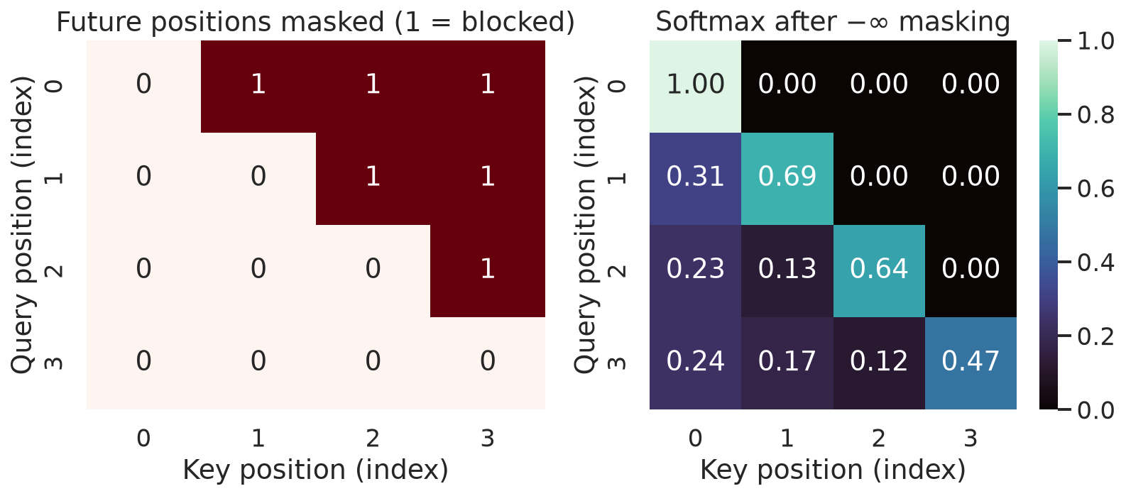
Figure 1. The upper-triangular blocked positions receive zero probability after score masking; the visible probabilities are normalized within each row.

3. Cross-attention and the decoder output

In Cross-Attention, the decoder representation \(D\) is [B, T, d] and the final encoder output \(E\) is [B, S, d]. Per head \(Q=DW_Q\), \(K=EW_K\), \(V_h=EW_V\); thus \(Q\) is [B, T, d_k], \(K\) is [B, S, d_k], \(V_h\) is [B, S, d_v], and \(QK^\top\) is [B, T, S]. Each query can weight every valid source key in ordinary offline translation. A source padding mask remains necessary; streaming variants may impose additional source restrictions. All decoder layers read the final encoder output through their own learned projections (PDF p. 24).

Concatenate \(h\) head outputs and project to [B, T, d]. The decoder's residual and normalization then precede the position-wise feed-forward network

The same FFN parameters act independently at every position; attention, not the FFN alone, mixes positions. For \(d=512\), \(f=2048\), this has \(2df+f+d=2,099,712\) parameters with biases. Top-layer states \(H\) [B, T, d] map to logits \(L=HW_D+b\) [B, T, V], \(W_D\) [d, V]; softmax across vocabulary yields next-token probabilities. At \(V=37,000\), the matrix has \(512\times37,000=18,944,000\) parameters, plus \(37,000\) if a bias is present. Transposed tying to an embedding matrix can share the weights; count shared parameters once and state vocabulary assumptions. The paper's shared embedding setup and approximate 65M base total are configuration-dependent (PDF pp. 24–25).

With standard biased full-width attention, one module has \(4d^2+4d\) parameters; two attention modules, FFN, and three affine layer norms give

At \(d=512,f=2048\), attention contributes 2,101,248, FFN 2,099,712, and norms 3,072, totaling 4,204,032. Six such layers have 25,224,192 parameters, excluding embeddings and output. The ebook's ~4M per layer is a rounded estimate, not an exact count; other bias, tying and normalization choices change totals. Encoder layers have one rather than two attention modules (PDF p. 25, Exam Tip).

The Dangerous Misconception: A decoder is an encoder with only an added mask. Why this is false: The original decoder also has a separate cross-attention sublayer and therefore another set of projections.

4. Sinusoidal position and relative offsets

Unmasked self-attention without positional signals is permutation equivariant: permuting input rows permutes output rows. In the original model, token embeddings are scaled by \(\sqrt d\) and added to fixed Sinusoidal Positional Encoding vectors before the first block. For even \(d\), with \(\omega_i=10000^{-2i/d}\),

At \(p=0\), all even channels are 0 and odd channels are 1; every component lies in \([-1,1]\) and \(\lVert PE(p)\rVert_2^2=d/2\). Lower-index pairs change faster across positions. For a fixed offset \(k\), the angle-addition identities give

Thus a block-diagonal linear map represents any fixed offset; learned attention is not guaranteed to exploit it. Furthermore \(PE(p)\cdot PE(p+k)=\sum_i\cos(k\omega_i)\) and squared distance is \(2\sum_i(1-\cos(k\omega_i))\). Distance is oscillatory, not generally monotonic in \(k\). The encoding can be evaluated at unseen positions, but this does not guarantee length extrapolation (PDF pp. 25–27).

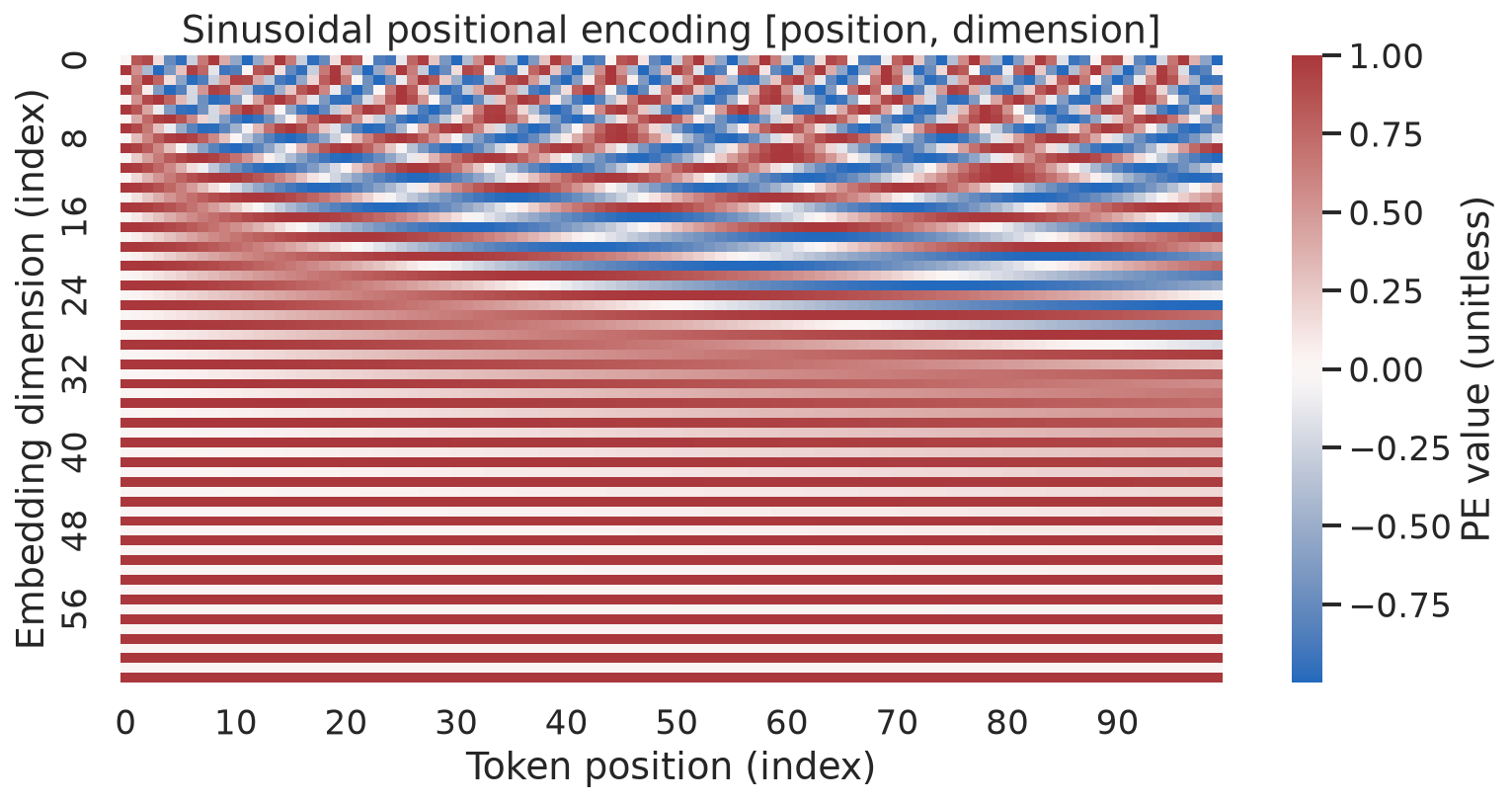
Figure 2. Across 100 positions and 64 channels, low-index sine–cosine pairs vary rapidly while higher-index pairs vary more slowly.

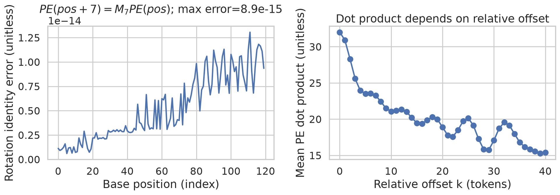
Figure 3. A fixed offset of 7 is represented by a two-dimensional rotation per frequency, up to floating-point error; encoding dot products vary with offset and need not decrease monotonically.

5. Residual connections and normalization

The original Transformer uses post-normalization at each of its three decoder sublayers:

with dropout on the sublayer output before addition during training. The operands have the same [B, T, d] shape. A bare residual \(x+F(x)\) has Jacobian \(I+J_F\), giving an additive gradient path, but the complete post-LN block also includes the LayerNorm Jacobian. A residual need not be small and does not guarantee nonvanishing gradients. Pre-LN instead uses \(x+F(\operatorname{LN}(x))\); it is a different wiring (PDF pp. 27–29).

For each token vector \(x\in\mathbb R^d\), Layer Normalization computes

The \(2d\) learned affine parameters are shared across tokens, whereas statistics are computed independently for each token and example. Ignoring \(\epsilon\), \(x=(1,2,3)\) has mean 2, variance \(2/3\), and normalized values \((-\sqrt{3/2},0,\sqrt{3/2})\). LayerNorm uses the same computation at training and evaluation. BatchNorm instead typically computes per-channel training statistics over batch and, for sequence BatchNorm, time; evaluation commonly uses running statistics. Padding can contaminate those statistics unless handled. Batch size 1 can still have multiple time observations.

Ebook correction (PDF p. 28): A single value in a BatchNorm training normalization set gives normalized activation zero and affine output \(\beta\), not the input; some implementations reject that case. This follows directly from the normalization equation and Ba et al.'s distinction between within-case and batch statistics. Ebook correction (PDF p. 29): Original BERT uses post-LN, not pre-LN; its original implementation applies LayerNorm after the residual addition. Neither post-LN instability without warmup nor pre-LN superiority is universal.

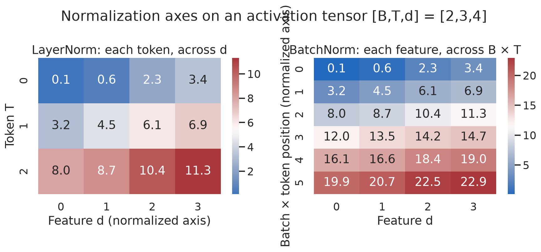
Figure 4. For [B,T,d]=[2,3,4], LayerNorm aggregates the four features of each token; BatchNorm pools batch and sequence observations for each feature.

6. Training objective and full data flow

For Label Smoothing under the uniform-mixture convention, \(q_i=(1-\varepsilon)\mathbf1[i=y]+\varepsilon/V\) and \(L=-\sum_i q_i\log p_i\). At \(V=5\), \(\varepsilon=0.1\), \(q_y=0.92\) and each other class receives 0.02. Another convention allocates \(\varepsilon\) exclusively to non-gold classes, giving \(q_y=0.9\); quote the convention. The original paper used \(\varepsilon=0.1\) and reported better accuracy and BLEU but worse perplexity; outcomes are empirical. Smoothed cross-entropy is not ordinary unsmoothed negative log-likelihood (PDF pp. 29–30).

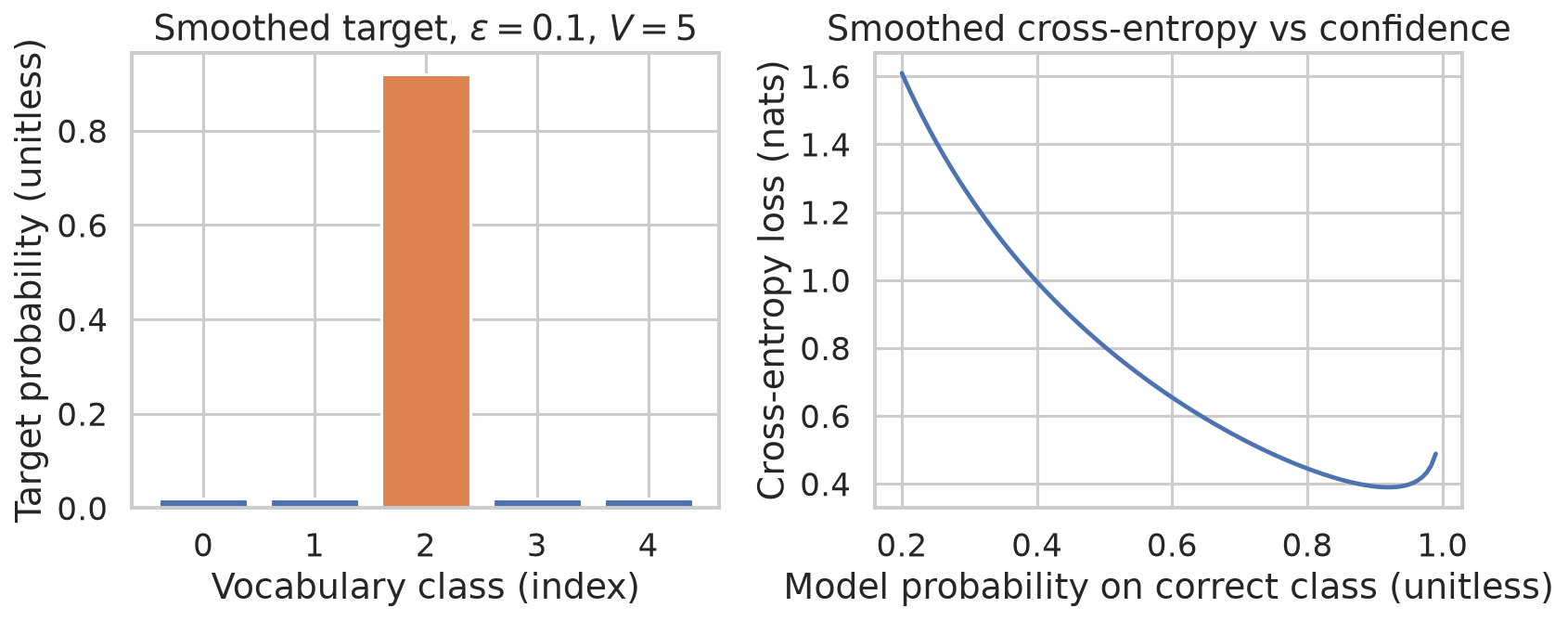
Figure 5. With five classes and smoothing 0.1, the gold class has target mass 0.92 and each alternative 0.02; the loss curve shows the effect of varying predicted confidence in the plotted example.

The original Learning-Rate Warmup schedule is

The two terms meet at \(s=w\): rate rises linearly to \(d^{-1/2}w^{-1/2}\) and then falls as \(s^{-1/2}\). For \(d=512\), the peak is approximately \(0.0006987712\). Adam applies adaptive parameter-wise scaling, so this schedule is not the actual magnitude of every update. The paper uses Adam \((\beta_1,\beta_2,\epsilon)=(0.9,0.98,10^{-9})\), and base dropout 0.1. Warmup is a training choice, not a universal stability proof.

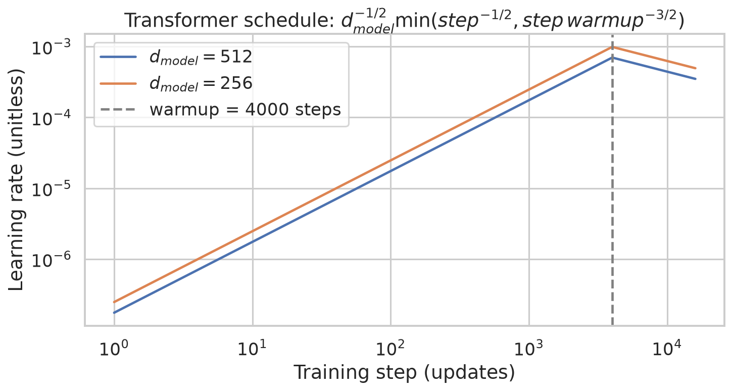
Figure 6. For widths 256 and 512, rates peak at step 4000 and decay thereafter; width 512 gives lower rates by a factor of \(1/\sqrt2\) at the same step.

The complete original data flow (PDF p. 29) is: source tokens → scaled embeddings plus positions → six encoder blocks of self-attention and FFN → final source memory; shifted target tokens → scaled embeddings plus positions → six decoder blocks, each with masked self-attention, source cross-attention, and FFN → vocabulary projection → softmax. Each sublayer is surrounded by residual addition and post-LN. Source and target may have different lengths. Training computes masked target positions in parallel; inference repeatedly appends a selected generated token until EOS or a length limit. Encoder–decoder attention is relevant to translation, summarization, speech transcription and image captioning when a model has source representations; decoder-only models omit the encoder and cross-attention.

7. Reproducible computational examples

The following source and stdout are reproduced verbatim from the supplied executed artifacts. Run from LLM/ with uv run python 'week 2/codeblocks/<filename>.py'. The examples are independent demonstrations rather than a trained translation system; outputs reflect the supplied execution environment.

Causal attention

Concept. A triangular score mask excludes future keys.

Code — 01_causal_mask.py.

import torch

torch.manual_seed(42)
scores = torch.tensor([[1.2,.5,2.1,-.3],[.2,1.,.8,1.1],[.4,-.2,1.4,.7],[.6,.3,-.1,1.3]])
mask = torch.triu(torch.ones(4,4,dtype=torch.bool), diagonal=1)
weights = torch.softmax(scores.masked_fill(mask, float("-inf")), dim=-1)
assert torch.all(weights.masked_select(mask) == 0)
print("causal mask (1=blocked):\n", mask.int())
print("masked attention weights:\n", weights)
print(f"future weight sum={weights.masked_select(mask).sum().item():.1f}")

Output.

causal mask (1=blocked):
 tensor([[0, 1, 1, 1],
        [0, 0, 1, 1],
        [0, 0, 0, 1],
        [0, 0, 0, 0]], dtype=torch.int32)
masked attention weights:
 tensor([[1.0000, 0.0000, 0.0000, 0.0000],
        [0.3100, 0.6900, 0.0000, 0.0000],
        [0.2344, 0.1286, 0.6370, 0.0000],
        [0.2352, 0.1743, 0.1168, 0.4737]])
future weight sum=0.0

Interpretation. The printed upper triangle sums to zero; remaining weights are row-normalized.

Cross-attention shapes

Concept. Different source and target lengths determine the rectangular attention matrix.

Code — 02_cross_attention_shapes.py.

import torch
import torch.nn as nn

torch.manual_seed(42)
B, Tdec, Tenc, D, H = 2, 3, 5, 16, 4
q, kv = torch.randn(B,Tdec,D), torch.randn(B,Tenc,D)
layer = nn.MultiheadAttention(D,H,batch_first=True,dropout=0.0)
y, a = layer(q,kv,kv,need_weights=True,average_attn_weights=False)
print(f"Q=[B,T_dec,d]=[{B},{Tdec},{D}], K=V=[B,T_enc,d]=[{B},{Tenc},{D}]")
print(f"weights [B,h,T_dec,T_enc]={list(a.shape)}; output={list(y.shape)}")
print("cross-attention has no causal mask over source positions")

Output.

Q=[B,T_dec,d]=[2,3,16], K=V=[B,T_enc,d]=[2,5,16]
weights [B,h,T_dec,T_enc]=[2, 4, 3, 5]; output=[2, 3, 16]
cross-attention has no causal mask over source positions

Interpretation. Four heads each connect three target queries to five source keys.

Sinusoidal encoding

Concept. The independent implementation is compared with the same mathematical formula.

Code — 03_sinusoidal_pe.py.

import numpy as np
import torch

def numpy_pe(pos, d):
    p = np.asarray(pos)[:,None]
    inv = 10000 ** (-2*np.arange(d//2)/d)
    phase = p*inv[None,:]
    out = np.empty((len(p),d)); out[:,0::2]=np.sin(phase); out[:,1::2]=np.cos(phase)
    return out

torch.manual_seed(42)
pos, d = np.arange(10), 16
manual = numpy_pe(pos,d)
pt = torch.zeros(10,d); p=torch.arange(10,dtype=torch.float32)[:,None]
i=torch.arange(0,d,2,dtype=torch.float32); phase=p*torch.exp(-np.log(10000)*i/d)
pt[:,0::2]=phase.sin(); pt[:,1::2]=phase.cos()
print(f"shape={manual.shape}; max |from scratch - formula implementation|={np.max(np.abs(manual-pt.numpy())):.8f}")
print(f"entry range=[{manual.min():.6f},{manual.max():.6f}]")

Output.

shape=(10, 16); max |from scratch - formula implementation|=0.00000011
entry range=[-0.989992,1.000000]

Interpretation. The maximum discrepancy is floating-point scale for this example.

Normalization axes

Concept. LayerNorm and BatchNorm aggregate different axes.

Code — 04_norm_axes.py.

import torch
import torch.nn as nn

torch.manual_seed(42)
x=torch.tensor([[[1.,2.,3.],[4.,5.,6.]],[[7.,8.,9.],[10.,11.,12.]]]) # [B,T,d]
ln=nn.LayerNorm(3,elementwise_affine=False)(x)
# BatchNorm1d on [B,C,T] normalizes each feature across B and T.
bn=nn.BatchNorm1d(3,affine=False,track_running_stats=False)(x.transpose(1,2)).transpose(1,2)
short=x[:1,:1,:]
print(f"[B,T,d]={list(x.shape)}; LN per-token means={ln.mean(-1)}")
print(f"BN changes with batch/padding population: feature-0 normalized values={bn[:,:,0]}")
print(f"single token LN output={nn.LayerNorm(3,elementwise_affine=False)(short).flatten()}")
# With one value per channel, training BatchNorm cannot estimate variance.
try:
    nn.BatchNorm1d(3)(torch.ones(1,3,1))
except ValueError as exc:
    print(f"BN on [1,3,1]: {str(exc).split('.')[0]}.")

Output.

[B,T,d]=[2, 2, 3]; LN per-token means=tensor([[0., 0.],
        [0., 0.]])
BN changes with batch/padding population: feature-0 normalized values=tensor([[-1.3416, -0.4472],
        [ 0.4472,  1.3416]])
single token LN output=tensor([-1.2247,  0.0000,  1.2247])
BN on [1,3,1]: Expected more than 1 value per channel when training, got input size torch.

Interpretation. The displayed per-token LayerNorm means vanish; the implementation rejects one BatchNorm observation.

Label smoothing

Concept. Uniform-mixture targets are evaluated by two cross-entropy calculations.

Code — 05_label_smoothing.py.

import torch
import torch.nn.functional as F

torch.manual_seed(42)
logits=torch.tensor([[0.2,-0.3,1.4,0.1]])
target=torch.tensor([2]); eps=.1; classes=4
prob=torch.softmax(logits,dim=-1)
y=torch.full_like(logits,eps/classes); y[0,target.item()]+=1-eps
manual=-(y*torch.log_softmax(logits,dim=-1)).sum(-1).mean()
torch_loss=F.cross_entropy(logits,target,label_smoothing=eps)
print(f"smoothed target={y.flatten().tolist()}")
print(f"manual loss={manual.item():.8f}; torch loss={torch_loss.item():.8f}; equal={torch.allclose(manual,torch_loss)}")

Output.

smoothed target=[0.02500000037252903, 0.02500000037252903, 0.9249999523162842, 0.02500000037252903]
manual loss=0.66827178; torch loss=0.66827178; equal=True

Interpretation. The two losses agree; the four-class gold target is 0.925 under this convention.

Warmup schedule

Concept. The original schedule varies with step and model width.

Code — 06_warmup_schedule.py.

for d in (512,256):
    warmup=4000
    print(f"d_model={d}")
    for step in (1,1000,4000,8000):
        lr=d**-0.5*min(step**-0.5,step*warmup**-1.5)
        print(f"  step={step:4d} lr={lr:.10f}")

Output.

d_model=512
  step=   1 lr=0.0000001747
  step=1000 lr=0.0001746928
  step=4000 lr=0.0006987712
  step=8000 lr=0.0004941059
d_model=256
  step=   1 lr=0.0000002471
  step=1000 lr=0.0002470529
  step=4000 lr=0.0009882118
  step=8000 lr=0.0006987712

Interpretation. The printed values peak at step 4000 and decline at 8000.

Decoder parameters

Concept. A biased decoder-layer formula is checked against the corresponding PyTorch module.

Code — 07_decoder_parameter_count.py.

import torch.nn as nn

d, ff, h = 512, 2048, 8
# Two attention modules (self + cross), FFN, and three affine LayerNorms.
attention = 2*(4*d*d+4*d)
feedforward = 2*d*ff+ff+d
norms = 6*d
formula=attention+feedforward+norms
layer=nn.TransformerDecoderLayer(d_model=d,nhead=h,dim_feedforward=ff,dropout=0.0,batch_first=True,norm_first=False,bias=True)
torch_count=sum(p.numel() for p in layer.parameters())
print(f"self+cross attention={attention:,}; FFN={feedforward:,}; 3 LayerNorms={norms:,}")
print(f"decoder layer formula={formula:,}; torch count={torch_count:,}; equal={formula==torch_count}")
print("Course shorthand ~4M; exact biased PyTorch module is 4.204M.")

Output.

self+cross attention=2,101,248; FFN=2,099,712; 3 LayerNorms=3,072
decoder layer formula=4,204,032; torch count=4,204,032; equal=True
Course shorthand ~4M; exact biased PyTorch module is 4.204M.

Interpretation. Both counts equal 4,204,032 under these settings.

Teacher forcing

Concept. The decoder receives shifted gold labels in teacher-forced training.

Code — 08_teacher_forcing.py.

import torch

torch.manual_seed(42)
truth=torch.tensor([1,2,3,4])
pred=torch.tensor([1,7,6,4])
# At each training step the next input is the gold previous token.
teacher_input=torch.cat([torch.tensor([0]),truth[:-1]])
# Free-running inference consumes the model's previous prediction.
free_input=torch.cat([torch.tensor([0]),pred[:-1]])
print(f"gold target={truth.tolist()}")
print(f"teacher-forced decoder input={teacher_input.tolist()}")
print(f"free-running decoder input={free_input.tolist()}")
print("teacher forcing exposes gold prefix; free-running errors can enter later inputs")

Output.

gold target=[1, 2, 3, 4]
teacher-forced decoder input=[0, 1, 2, 3]
free-running decoder input=[0, 1, 7, 6]
teacher forcing exposes gold prefix; free-running errors can enter later inputs

Interpretation. The free-running prefix contains generated errors rather than the gold prefix.

8. Failure modes and handoff

Masking only padding does not enforce causality; masking only future target keys does not remove source padding. Misaligned targets leak labels even with a triangular mask. A source attention matrix has \(T\) query rows and \(S\) key columns, so confusing the two silently produces wrong dimension calculations. A PE defined for arbitrary positions does not establish out-of-distribution generalization. Distinguish normalization statistics from learnable affine parameters, and count shared matrices once. Week 3 continues from this architecture to decoder-only language modelling and its input and prediction conventions: Week 3: Language Modelling, GPT-1, and Transfer.

9. References and source notes

• Vaswani, A., Shazeer, N., Parmar, N., Uszkoreit, J., Jones, L., Gomez, A. N., Kaiser, Ł., and Polosukhin, I. (2017). “Attention Is All You Need.” Advances in Neural Information Processing Systems 30. doi:10.48550/arXiv.1706.03762. Contribution: original architecture, positional encoding, training and base configuration.
• Ba, J. L., Kiros, J. R., and Hinton, G. E. (2016). “Layer Normalization.” arXiv preprint. doi:10.48550/arXiv.1607.06450. Contribution: within-example normalization and affine parameters.
• Devlin, J., Chang, M.-W., Lee, K., and Toutanova, K. (2019). “BERT: Pre-training of Deep Bidirectional Transformers for Language Understanding.” NAACL-HLT, 4171–4186. doi:10.18653/v1/N19-1423. Contribution: BERT architecture; the original implementation shows post-residual normalization.
• Local course transcript ../sources/ebook/week-2-transcript.md and ../sources/ebook-discrepancies.md: page references, exam tips, and flagged claims. Executed artifacts and captions follow codeblocks/MANIFEST.md.