Week 3 in Plain Language: Predicting the Next Word, GPT-1 and Pre-train then Fine-tune
Explain-like-I'm-12 version of the full Week 3 notes. Exam wording lives in the exam-focused guide and the real routed questions in the Week 3 question bank. If the decoder, the causal mask or teacher forcing feel shaky, revisit Week 2 in plain language first. Everything sits under the Knowledge Map.
The big idea of Week 3. A language model is a machine that, given the words so far, gives a probability to every possible next word. Chain those guesses together and you get a probability for a whole sentence. GPT-1 learns this guessing game from huge amounts of unlabelled text (pre-training), then gets a small amount of extra practice on a labelled task (fine-tuning). The same network, with a little reformatting of the input, then solves many different tasks.
Notation: B = batch size, T = sequence length, d = model width, f = feed-forward width, V = vocabulary size, C = number of classes.
1. What a language model predicts, and the chain rule
Think of your phone's keyboard suggestion. After "I like" it ranks "tea", "you", "pizza" and so on. A language model does this with proper probabilities.
To score a whole sentence, multiply the next-word probabilities along the way. This is the chain rule of probability, and it is always true:
Hand-check (executed example, 02_chain_rule.py). Sentence <s> I like tea, with start symbol <s>:
| Step | Context | Probability of the real next word |
|---|---|---|
| 1 | <s> |
\(0.4\) for "I" |
| 2 | <s> I |
\(0.6\) for "like" |
| 3 | <s> I like |
\(0.5\) for "tea" |
Product: \(0.4\times0.6\times0.5=0.12\), and \(\log 0.12=-2.120264\). If the model only used the previous word (a bigram shortcut) and its factors were \(0.4,0.3,0.2\), the product would be \(0.024\). In this toy the full-history sentence is \(0.12/0.024=5\) times more likely. That is a property of these made-up numbers, not a law that more context always wins.
Taking \(-\log\) of each factor turns the product into a sum of per-word "costs": \(0.9163+0.5108+0.6931\) for the full-history factors, versus \(0.9163+1.204+1.6094\) for the bigram ones (06_chain_summary.py).
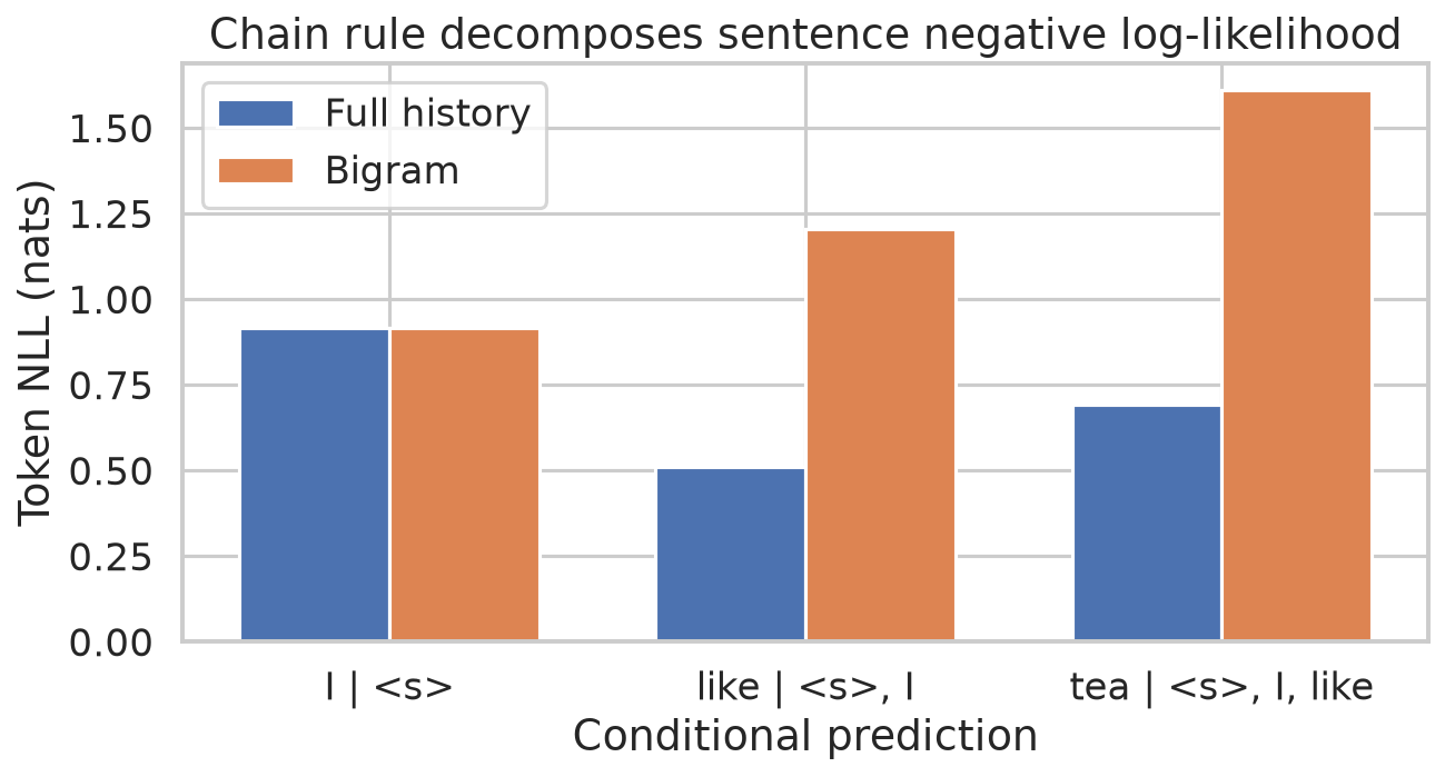
Figure 1. Full-history probabilities 0.4, 0.6 and 0.5 give token losses 0.916, 0.511 and 0.693 nats. The toy bigram's later probabilities 0.3 and 0.2 give larger losses.
Mistakes people make.
- "The chain rule assumes words are independent." No. The chain rule is exact and keeps the dependence on earlier words. Replacing \(p(w_i\mid w_{<i})\) by plain \(p(w_i)\) is a separate, wrong independence assumption.
- "A high sentence probability means the sentence is true." No. It only measures fit to what the model learned, not facts.
- Inventing a probability the question did not give you. If a tree lacks the needed branch, the honest answer is "insufficient information".
Where the exam asks this
- 2024 T3 Quiz 1, Q285: probability of the first predicted word given
[Start]. Derived answer: 0.41. - 2024 T3 Quiz 1, Q286: multiply the branch probabilities of a sentence, then scale by 1000. Derived answer: approximately 1.637.
- 2025 T1 Quiz 1, Q119 and Q120: two-word and five-word joint probabilities scaled by 100. Derived answers: about 2.4390244 for both.
- 2026 T2 Quiz 1, Q10: joint probability of "You eat apples". Derived answer: 0.18.
- 2026 T2 Quiz 1, Q12: derived answer -1, because the given tree does not supply the asked conditional.
- Also routed here: 2024 T3 Quiz 1, Q287, 2025 T1 Quiz 1, Q118, Q121 (derived: "broken" is the most likely next token), 2026 T2 Quiz 1, Q11 (marked ambiguous, no answer quoted).
2. Ways to build the next-word predictor (briefly)
The chain rule says what to compute, not which machine computes it. Three ways to supply \(p(w_i\mid w_{<i})\):
| Machine | How it handles the past |
|---|---|
| n-gram | Looks only at the last \(n-1\) words and counts how often they occurred (with smoothing for unseen cases) |
| RNN | Squeezes the past into one running summary (its state), updated word by word, so it is sequential |
| Causal Transformer | Attention over the allowed earlier words, plus position information; its window is finite |
The ebook also sorts models into encoder-only (fill in masked words), decoder-only (predict left to right) and encoder-decoder (translate-style). Masked-word prediction is a different question from left-to-right next-word prediction. No exam question is routed to this section, so just know the three machines.
3. Perplexity: how surprised is the model?
Perplexity is not defined in the ebook. The notes add it from the standard definition, because it is the usual way to report a language model's quality.
Perplexity answers: "on average, the model behaves as if it were choosing among this many equally likely words." Formally it is the exponential of the average per-word cost:
Lower is better (less surprised), on the same text with the same tokenisation.
Hand-check (executed example, 01_perplexity.py). The model gave the three real words probabilities \(0.8,\,0.5,\,0.25\).
- Per-word costs: \(-\ln0.8=0.2231\), \(-\ln0.5=0.6931\), \(-\ln0.25=1.3863\).
- Their mean is the cross-entropy: \(0.767528\) nats/token.
- \(\exp(0.767528)=2.154435\).
- Cross-check: the product of the probabilities is \(0.8\times0.5\times0.25=0.1\), and \(0.1^{-1/3}=2.1544\). Perplexity is the reciprocal geometric mean of the probabilities.
Sanity anchor: if a model gives every one of 4 words probability \(1/4\), the mean cost is \(\ln4\) and the perplexity is exactly \(4\).
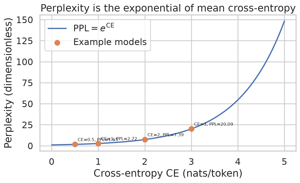
Figure 2. Cross-entropies 0.5, 1, 2 and 3 nats/token correspond to perplexities of approximately 1.65, 2.72, 7.39 and 20.09.
Mistakes people make.
- Comparing perplexities from models with different tokenisers or different test text. They are not directly comparable.
- Thinking low perplexity proves the model is factual. It does not.
- Forgetting that one zero-probability word makes the perplexity infinite.
Where the exam asks this. No routed Week 3 question is specifically about perplexity; the topic it belongs to is the one in section 1, and the exam there tests the joint-probability multiplication. Treat perplexity as supporting intuition. See Perplexity and Language-Modelling Objective.
4. Causal language model: one pass, every next-word loss
Causal means "no peeking at the future". A GPT block is the Week 2 decoder block with the cross-attention removed: masked self-attention, then a feed-forward layer, with residual connections and layer normalisation. Each position may look at itself and earlier positions only; the future gets \(-\infty\) before the softmax:
The final states [T, d] are multiplied by the transposed token table [d, V] to give scores [T, V]; softmax turns each row into a probability over the vocabulary.
Why one forward pass is enough. The state at position \(j\) predicts the token at position \(j+1\), and the mask guarantees it never saw later tokens. So all \(T\) predictions are valid at once, and all their losses can be added up from a single pass. The labels are the inputs shifted by one.
Hand-check 1 (shift). Input [BOS, a, b] with real continuation c. The BOS state predicts a, the a state predicts b, the b state predicts c. Targets: [a, b, c].
Hand-check 2 (mask size). For 5 positions the blocked future pairs number \(4+3+2+1=10=5\cdot4/2\).
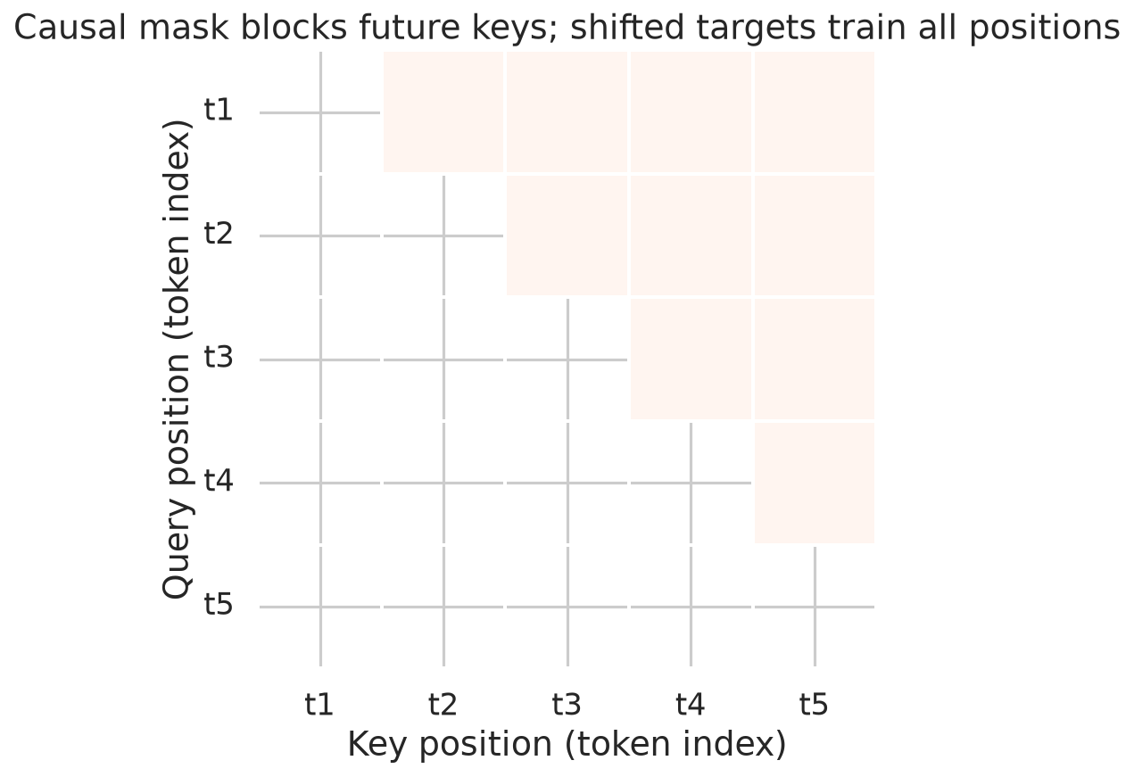
Figure 3. For five positions, the upper triangle blocks 10 future query-key pairs; the diagonal and earlier positions stay accessible.
Hand-check 3 (executed, 03_causal_and_shift.py). Take score rows [2, 0, -1] and [0, 1, 2] with targets 1 and 2 (the shifted labels). The costs are \(\ln(e^2+1+e^{-1})-0=2.1698\) and \(\ln(1+e+e^2)-2=0.4076\). Their mean is \(1.288726\), matching the output. The same script changes only future tokens and finds the earlier logits move by \(0.00000000\).
Mistakes people make.
- "The mask alone stops cheating." No. The current token sits in the stream through residual connections, so you must also shift the labels.
- "A decoder-only model cannot classify." It can: the last position can look at everything before it and feed a classifier. Whether it summarises well is not guaranteed.
- "The last state has seen the future." No, it sees only what came before it.
Where the exam asks this
- 2025 T2 Quiz 1, Q140: true statements about causal language modelling. Derived answer: A and B (attends to past and current tokens only; trained by next-token prediction).
- 2025 T3 End Term AN, Q23: derived answer B, predict \(x_{t+1}\) from earlier tokens only.
- 2025 T3 End Term FN, Q23: derived answer A and B.
- 2026 T1 Quiz 2, Q13: is the shown attention matrix causal? Derived answer: false.
- 2026 T2 Quiz 1, Q13: parts of a GPT decoder layer. Derived answer: A, B and E (masked attention, feed-forward, add and norm; no cross-attention, no RNN).
- Also routed here: 2024 T1 Quiz 1, Q193, 2024 T1 End Term AN, Q149 and 2024 T1 End Term FN, Q202 (no derived answer is quoted for these).
5. GPT-1: the architecture and the pre-train / fine-tune idea
GPT-1 stacks decoder blocks. The numbers to remember:
| Piece | Value |
|---|---|
| Blocks | 12 |
Hidden width d |
768 |
| Attention heads | 12, each of width 64 |
Feed-forward width f |
3,072 |
| Context length | 512 |
| Positions | learned (absolute) position embeddings |
| Activation | GELU |
Pre-train / fine-tune, as a school analogy. First the model reads a huge pile of ordinary books (BookCorpus, no labels needed) just by playing the next-word game. That teaches it grammar and a lot about the world. Then it gets a short, focused course on one labelled task, such as spotting sentiment. The reading is the pre-training, the course is the fine-tuning. Fine-tuning starts from the pre-trained weights, not from scratch.
Mistakes people make.
- Saying all parameters are randomly initialised during fine-tuning. They start from the pre-trained values (only the new task head is fresh).
- Forgetting that fine-tuning normally needs a labelled dataset, while pre-training does not.
Where the exam asks this
- 2024 T1 End Term AN, Q144: what "GPT" stands for. Derived answer: Generative Pre-trained Transformer.
- 2024 T3 End Term AN, Q193: GPT-1 facts. Derived answer: A and B (decoder-only; absolute positions).
- 2025 T2 Quiz 1, Q141: why Transformer LLMs are popular. Derived answer: A and D (parallel processing; fine-tuning for many tasks).
- Also routed here: 2025 T1 Quiz 1, Q108 (marked ambiguous, no answer quoted).
See GPT-1 Architecture and Pretrain–Fine-tune Paradigm.
6. Counting GPT-1's parameters: the famous 117M
Count what must be stored. With \(V=40{,}478\), \(T=512\) (positions), \(d=768\), \(f=3072\), \(L=12\) (executed in 04_gpt1_parameters.py):
| Part | Formula | Count |
|---|---|---|
| Token + position tables | \((V+T)d\) | 31,480,320 |
| Attention (Q, K, V, output, with biases) | \(L(4d^2+4d)\) | 28,348,416 |
| Feed-forward (two layers, with biases) | \(L(2df+f+d)\) | 56,669,184 |
| Two LayerNorms per block | \(L\cdot4d\) | 36,864 |
| Total | 116,534,784 |
That is 116.5 million, which rounds to 117M. Check the first row by hand: \(40{,}478\times768=31{,}087{,}104\) for tokens, \(512\times768=393{,}216\) for positions, total \(31{,}480{,}320\). One feed-forward layer: weights \(2\cdot768\cdot3072=4{,}718{,}592\), biases \(3072+768=3{,}840\), total \(4{,}722{,}432\); times 12 gives \(56{,}669{,}184\).
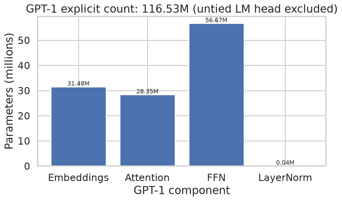
Figure 4. The tied convention gives 31,480,320 embedding, 28,348,416 attention, 56,669,184 feed-forward and 36,864 LayerNorm parameters, totalling 116,534,784.
Two caveats the notes insist on.
- The output layer is not counted twice. GPT-1 reuses ("ties") the token table, transposed, to make the final scores. Counted once. An untied output matrix would add \(40{,}478\times768=31{,}087{,}104\) more.
- Vocabulary size vs merges. The paper's 40,000 is the number of byte-pair merge operations; the ebook configuration used here has 40,478 vocabulary entries. These are different quantities, so do not use 40,000 as the vocabulary size.
The total also depends on convention (biases, LayerNorm, tying), so say which convention you use. The ebook's mnemonic "31 + 27 + 56 = 114M" is a rough memory aid that understates the sum; trust the executed 116,534,784.
Mistakes people make.
- Adding a separate vocabulary-sized output matrix to the 117M.
- Forgetting the feed-forward biases, or mixing "weights only" with "weights and biases" questions.
- Using memorised GPT-1 numbers when the question gives its own dimensions.
Where the exam asks this
- 2026 T1 Quiz 1, Q16: token embedding matrix size. Derived answer: option A, 30,720,000 (which equals \(40{,}000\times768\)).
- Q17: positional matrix. Derived answer: B, 393,216 (the same \(512\times768\) as above).
- Q19: output projection weights only. Derived answer: C, 589,824.
- Q20: full FFN with biases. Derived answer: C, 4,722,432.
- 2024 T1 Quiz 2, Q135: decoder-only counts (embedding and output excluded). Derived answer: D, all the same.
- Also routed here: 2026 T1 Quiz 1, Q18 (ambiguous, no answer quoted) and 2024 T3 Quiz 1, Q289.
Always use the dimensions printed in the question, not GPT-1's. (Q20's option C, 4,722,432, happens to equal the per-block GPT-1 feed-forward count computed above.)
7. Pre-training objective and teacher forcing
Pre-training maximises the sum of log-probabilities of the real next words. Machine learners prefer to minimise, so we minimise its negative, which is the ordinary cross-entropy loss: \(-\sum_i\log\hat p_i(u_i)\).
Teacher forcing means the inputs are the real text, and the labels are the same text shifted by one. Because the real prefix is always supplied, every position can be computed at the same time with the mask. At generation time no real text exists: each chosen word is fed back as input, so generation is one word at a time. Fast parallel training and slow sequential writing are both true.
Hand-check (number of labels). A sequence of length 1024 without a start token supplies \(1023\) next-word labels. With a batch of 32 such sequences: \(32\times1023=32{,}736\) targets, the derived answer to 2025 T3 Quiz 1, Q189 below. Padding and an unscored start token must not be counted.
Mistakes people make.
- "Training is sequential like generation." Transformer training scores all positions in parallel.
- "Teacher forcing computes loss only on wrong tokens." No, every position counts.
- Thinking only words in the batch get gradient. With a full softmax, even absent words sit in the denominator and get updates; with tied weights they can also reach the input table.
Where the exam asks this
- 2025 T3 End Term AN, Q24: how teacher forcing relates to the loss. Derived answer: C, each prediction is conditioned on the ground-truth prefix.
- 2025 T3 Quiz 1, Q189: number of next-token targets in a full batch. Derived answer: 32,736.
- 2024 T3 End Term AN, Q177: do rare vocabulary embeddings get updated under shared weights? Derived answer: B, they can be.
- 2024 T3 End Term FN, Q194 (derived: A, B, D) and 2024 T1 Quiz 1, Q194 (ambiguous, no answer quoted).
See Teacher Forcing.
8. Fine-tuning and its loss
After pre-training, add a small head (for classification, a layer mapping the final position's state to C class scores, so logits are [B, C]) and train everything on labelled examples. Why the last position? Because of the causal mask it is the only one that has looked at the whole input.
The paper trains with a combined objective:
where \(L_2\) is the supervised log-likelihood (the task) and \(L_1\) is the language-model log-likelihood (the old next-word game, kept as a helper). Equivalently, minimise their negatives. The paper reports that the helper improves generalisation and speeds convergence.
Hand-check. Take \(L_2=-0.7\), \(L_1=-2\), \(\lambda=0.1\). Then \(L_3=-0.7+0.1(-2)=-0.9\), so the loss to minimise is \(0.9\).
Mistakes people make.
- Reading \(L_1\) and \(L_2\) as L1 and L2 weight penalties. They are log-likelihoods. The notes' toy script (
05_finetuning_loss.py) uses real norms on purpose to show the contrast: task loss \(0.7\) plus \(0.5\times5.25\) plus \(0.1\times3.5\) gives \(3.675\). That is a norm penalty, not GPT-1's objective. - Claiming the helper loss is proven to prevent forgetting. The paper's evidence is better generalisation and faster convergence, not that claim.
Where the exam asks this
- 2026 T2 Quiz 2, Q9: why use the final input token's state. Derived answer: D, causal attention lets the final token's representation depend on the whole preceding input.
- 2024 T3 End Term FN, Q194: true statements about GPT. Derived answer: A, B and D (labelled data is generally needed for fine-tuning).
- Also routed here: 2024 T1 Quiz 1, Q194 and 2025 T1 Quiz 1, Q108 (both ambiguous, no answer quoted).
9. Task-specific input formats
The trick: instead of redesigning the network for each task, serialise the task into one token sequence with special markers, then reuse the same network.
| Task | Sequence layout and what is scored |
|---|---|
| Sentiment / classification | Start, text, end; classify the end position's state |
| Entailment | Start, premise, delimiter, hypothesis, end; classify the pair's relation |
| Similarity | Run both sentence orders and combine, since the task is symmetric |
| Multiple choice | Context, question and each candidate as a separate sequence; shared network gives one score per candidate; softmax over the candidates |
| Generation | Give a prefix and continue it word by word |
Hand-check. Three answer choices, all with equal scores, give each choice probability \(1/3\). If one score is larger, that choice wins. The delimiter is a boundary marker, not the answer.
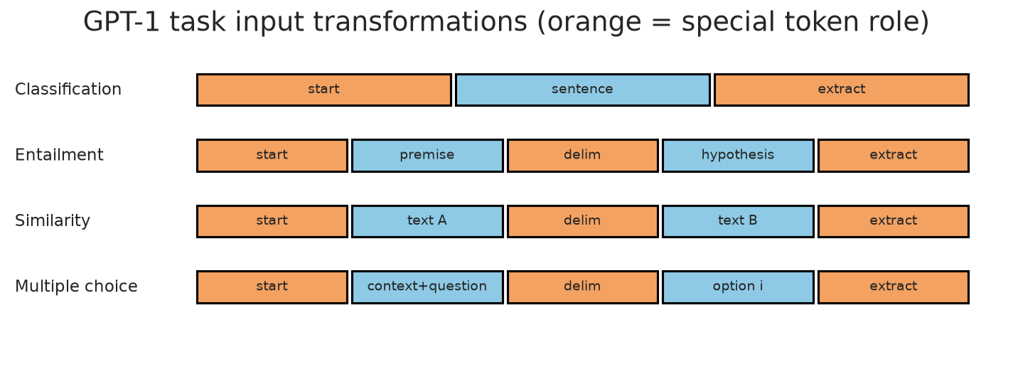
Figure 5. The four diagrams locate start and delimiter markers and the extracted representation for classification, entailment, similarity and multiple-choice inputs.
Where the exam asks this
- 2026 T2 Quiz 2, Q8: purpose of the delimiter in entailment. Derived answer: B, to separate premise and hypothesis.
See Task-Specific Input Transformations.
The answers quoted above are derived study aids produced by the study team, not official answer keys. Where a record is marked ambiguous in the bank, no answer is quoted here.
Check yourself
- Conditionals are \(0.5,\,0.5,\,0.2\). What is the sentence probability and its perplexity over those 3 tokens?
- Input
[BOS, x, y], original continuationz. What are the three targets, and why is a mask alone not enough? - How many future pairs does the causal mask block for 4 positions?
- With \(V=40{,}478\) and \(d=768\), how many parameters would untying the output matrix add, and why does GPT-1 not pay this?
- In \(L_3=L_2+\lambda L_1\), what are \(L_2\) and \(L_1\)? Compute \(L_3\) for \(L_2=-1.0\), \(L_1=-3.0\), \(\lambda=0.5\).
Answers
- \(0.5\times0.5\times0.2=0.05\). Perplexity \(=0.05^{-1/3}\approx2.71\) (the reciprocal geometric mean of the probabilities).
- Targets
[x, y, z]. The current token still reaches its own state through the residual path, so labels must also be shifted by one. - \(3+2+1=6=4\cdot3/2\).
- \(40{,}478\times768=31{,}087{,}104\). GPT-1 reuses the transposed token table as the output matrix, so it is stored and counted once.
- \(L_2\) is the supervised (task) log-likelihood; \(L_1\) is the auxiliary language-model log-likelihood. \(L_3=-1.0+0.5(-3.0)=-2.5\), so the loss to minimise is \(2.5\).
Bridge to Week 4
Week 3 taught the model to produce a probability for the next word. It did not say which word to actually write. Week 4 in plain language turns those probabilities into generated text (greedy, beam search, sampling) and contrasts left-to-right modelling with masked-word modelling. Look back at Week 2 for the decoder mechanics, and see the formal treatment in the Week 3 notes, the exam-focused guide and the question bank.